Diagnostic plots for galamm objects

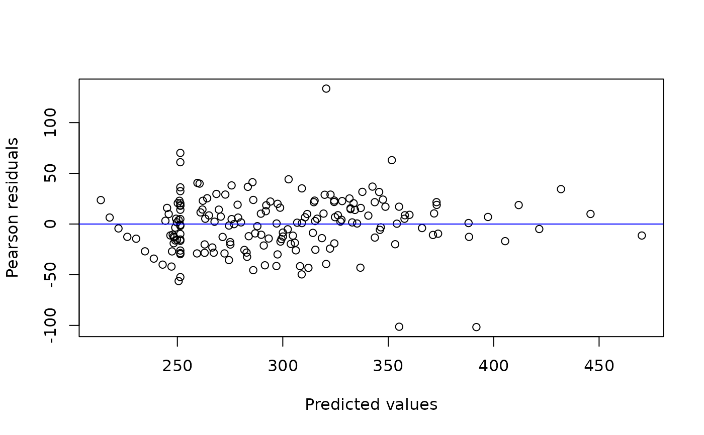
This function provides diagnostic plots for models fitted with galamm(). See the residuals.galamm() function for definition of the residuals being used.

Usage

# S3 method for class 'galamm'
plot(x, form = resid(., type = "pearson") ~ fitted(.), abline = NULL, ...)

Arguments

x

An object of class galamm returned from galamm.

form

An option formula specifying the desired type of plot. Conditioning variables are specified with a vertical bar.

abline

An optional numeric vector specifying the intercept and slope of a line to be added to the plot.

...

Optional arguments passed on to the plot functions in the lattice package.

Value

A plot is displayed.

Details

The interface of this function is designed to be similar to the plot.merMod function from lme4 (Bates et al. 2015) .

References

Bates DM, Mächler M, Bolker B, Walker S (2015). “Fitting Linear Mixed-Effects Models Using Lme4.” Journal of Statistical Software, 67(1), 1–48. ISSN 1548-7660, doi:10.18637/jss.v067.i01 .

See also

residuals.galamm() for extracting residuals and plot() for the generic function.

Other diagnostics: qqmath.galamm()

Author

Douglas Bates, Martin Maechler, Ben Bolker, and Steven Walker, with modifications by Øystein Sørensen.

Examples

## Linear mixed model example from lme4
data("sleepstudy", package = "lme4")
mod <- galamm(Reaction ~ Days + (Days | Subject), data = sleepstudy)

# Diagnostic plot of Pearson residuals versus fitted values
plot(mod)


# Include a straight line at zero
plot(mod, abline = c(0, 0))


# Diagnostic plot of Pearson residuals versus fitted values per subject
plot(mod, form = resid(., type = "pearson") ~ fitted(.) | Subject)


# Residuals plotted against time with a straight line at zero
plot(mod, form = resid(., type = "pearson") ~ Days, abline = c(0, 0))


# Residuals plotted against time per subject with a straight line at zero
plot(mod, form = resid(., type = "pearson") ~ Days | Subject,
     abline = c(0, 0))


# Box plot of residuals by Subject
plot(mod, Subject ~ resid(., scaled=TRUE))


## Logistic mixed model example from lme4
data("cbpp", package = "lme4")
mod <- galamm(cbind(incidence, size - incidence) ~ period + (1 | herd),
              data = cbpp, family = binomial)

# Diagnostic plot using Pearson residuals
plot(mod)


# Diagnostic plot using deviance residuals
plot(mod, resid(., type = "deviance") ~ fitted(.))


# Diagnostic plot per herd
plot(mod, resid(., type = "deviance") ~ fitted(.) | herd)


## Linear mixed model with factor structures
# See vignette on linear mixed models with factor structures for details
data(KYPSsim, package = "PLmixed")
KYPSsim <- KYPSsim[KYPSsim$sid < 100, ]
KYPSsim$time <- factor(KYPSsim$time)

loading_matrix <- rbind(c(1, 0), c(NA, 0), c(NA, 1), c(NA, NA))
factors <- c("ms", "hs")
load_var <- "time"
form <- esteem ~ time + (0 + ms | mid) + (0 + hs | hid) + (1 | sid)

mod <- galamm(formula = form, data = KYPSsim, factor = factors,
              load_var = load_var, lambda = loading_matrix)

# Pearson residuals plotted against fitted value
plot(mod)


# Actual value plotted against fitted value with a line crossing the diagonal
plot(mod, form = esteem ~ fitted(.), abline = c(0, 1))