Generalized Linear Mixed Models with Factor Structures
Source:vignettes/glmm_factor.Rmd
glmm_factor.RmdThis vignette describes how galamm can be used to
estimate generalized linear mixed models with factor structures. Such
models are an instance of the generalized linear latent and mixed models
(GLLAMM) framework described by Rabe-Hesketh,
Skrondal, and Pickles (2004).
The R package PLmixed (Rockwood and Jeon
2019) estimates such models using a profile likelihood
algorithm initially proposed by Jeon and
Rabe-Hesketh (2012).
The models are also a special case of generalized additive latent and
mixed models (GALAMM), and in galamm these models are estimated using a
more direct algorithm described in Sørensen,
Fjell, and Walhovd (2023).
As for the vignette on linear mixed models, we thank Rockwood and Jeon (2019) for creating the PLmixed package, from which we take example datasets, and on which we have based the formula syntax of galamm.
Model with Binomially Distributed Responses
We use a simulated dataset from the PLmixed package for this example. The observations are binomial responses representing an ability measurement. The first few lines are shown below.
library(PLmixed)
head(IRTsim)
#>     sid school item y
#> 1.1   1      1    1 1
#> 1.2   1      1    2 1
#> 1.3   1      1    3 1
#> 1.4   1      1    4 0
#> 1.5   1      1    5 1
#> 2.1   2      1    1 1
Each student is identified by a student id sid, and each
school with a school id given by the school variable. For
each student, five item measurements have been made. We assume that the
student’s performance depends both on the students ability as well as on
the school the student attends. Having the outline of GALAMMs from the
introductory
vignette in mind, we assume a binomial response model with a logit
link, yielding for the
th
measurement of the
th
student in the
th
school,
The latent variable vector is given by , where the last element is the effect of the school which the th student attends. The nonlinear predictor is given by
where is a vector containing dummy variables for items, is a latent variable describing the underlying ability of student , and is a latent variable describing the effect of school . The factor loading describes how the sum of the two latent variables impacts the nonlinear predictor, and hence the probability of correct response. We note that using a common for two latent variables like this is not necessarily a good model, but it makes this introductory example easier to follow. We will extend the model later.
The structural model is simply
where denotes a bivariate normal distribution with mean zero covariance matrix . The covariance matrix is assumed to be diagonal.
IRTsim$item <- factor(IRTsim$item)We confirm that item has five levels. This means that
is a vector with five elements.
table(IRTsim$item)
#>
#>   1   2   3   4   5
#> 500 500 500 500 500
For identifiability, we fix the first element of
to one. The rest will be freely estimated. We do this by defining the
following matrix. Any numeric value implies that the element is fixed,
whereas NA implies that the element is unknown, and will be
estimated.
(loading_matrix <- matrix(c(1, NA, NA, NA, NA), ncol = 1))
#>      [,1]
#> [1,]    1
#> [2,]   NA
#> [3,]   NA
#> [4,]   NA
#> [5,]   NA
We fit the model as follows:
mod <- galamm(
  formula = y ~ item + (0 + ability | school / sid),
  data = IRTsim,
  family = binomial,
  load_var = "item",
  factor = "ability",
  lambda = loading_matrix
)
A couple of things in the model formula are worth pointing out. First
the part (0 + ability | school / sid) in the model formula
specifies that student ability varies between students within schools.
It corresponds to the term
in the mathematical specification of the model. The variable
ability is not part of the IRTsim dataframe,
but is instead specified in the argument
factor = "ability". The argument
load_var = "item" specifies that all rows in the dataframe
with the same value of “item” should get the same element of
,
and hence it defines the dummy variable
.
Finally, lambda = loading_matrix provides the matrix of
factor loadings. Note that we must explicitly add a zero in
(0 + ability | school / sid) to avoid having a random
intercept estimated in addition to the effect for each value of “item”;
such a model would not be identified. The fixed effect part of the model
formula, which is simply item, specifies the term
.
We can start by inspecting the fitted model:
summary(mod)
#> GALAMM fit by maximum marginal likelihood.
#> Formula: y ~ item + (0 + ability | school/sid)
#>    Data: IRTsim
#>
#>      AIC      BIC   logLik deviance df.resid
#>   2966.4   3030.5  -1472.2   2372.3     2489
#>
#> Scaled residuals:
#>     Min      1Q  Median      3Q     Max
#> -2.8884 -0.7335  0.4266  0.6235  3.0410
#>
#> Lambda:
#>         ability     SE
#> lambda1  1.0000      .
#> lambda2  0.7370 0.1456
#> lambda3  0.9351 0.1872
#> lambda4  0.6069 0.1261
#> lambda5  0.5860 0.1163
#>
#> Random effects:
#>  Groups     Name    Variance Std.Dev.
#>  sid:school ability 1.466    1.211
#>  school     ability 1.300    1.140
#> Number of obs: 2500, groups:  sid:school, 500; school, 26
#>
#> Fixed effects:
#>             Estimate Std. Error z value Pr(>|z|)
#> (Intercept)   0.5112     0.2617   1.953 0.050777
#> item2         0.3256     0.1791   1.818 0.069068
#> item3        -0.4491     0.1623  -2.768 0.005644
#> item4         0.4930     0.1924   2.562 0.010402
#> item5         0.4585     0.1922   2.385 0.017067
The fixef method lets us consider the fixed effects:
fixef(mod)
#> (Intercept)       item2       item3       item4       item5
#>   0.5112006   0.3255941  -0.4491070   0.4929827   0.4584897
We can also get Wald type confidence intervals for the fixed effects.
confint(mod, parm = "beta")
#>                    2.5 %     97.5 %
#> (Intercept) -0.001727334  1.0241286
#> item2       -0.025430062  0.6766183
#> item3       -0.767138526 -0.1310755
#> item4        0.115869898  0.8700955
#> item5        0.081749228  0.8352303
We can similarly extract the factor loadings.
factor_loadings(mod)
#>           ability        SE
#> lambda1 1.0000000        NA
#> lambda2 0.7370254 0.1455782
#> lambda3 0.9351105 0.1872049
#> lambda4 0.6069065 0.1260943
#> lambda5 0.5859914 0.1162977
And we can find confidence intervals for them. Currently, only Wald type confidence intervals are available. Be aware that such intervals may have poor coverage properties.
confint(mod, parm = "lambda")
#>             2.5 %    97.5 %
#> lambda1 0.4516974 1.0223534
#> lambda2 0.5681956 1.3020254
#> lambda3 0.3597662 0.8540468
#> lambda4 0.3580520 0.8139307
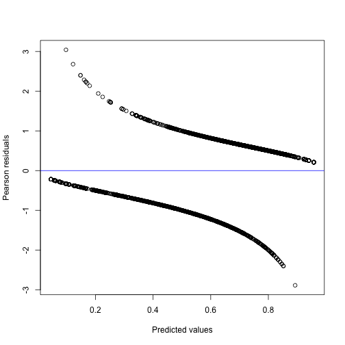
We can also make a diagnostic plot, where we use deviance residuals since these are more useful for logistic regression models. The division into two parts is a consequence of the binary outcomes.

Binomial Model with Multiple Trials
We now show how the model studied above can be extended to handle binomially distributed data with multiple trials. We simulate such data by computing predictions from the model fitted above, and drawing binomial samples with multiple trials.
set.seed(1234)
dat <- IRTsim
dat$trials <- sample(1:10, nrow(dat), replace = TRUE)
dat$y <- rbinom(
  n = nrow(dat), size = dat$trials,
  prob = plogis(fitted(mod))
)
head(dat)
#>     sid school item y trials
#> 1.1   1      1    1 8     10
#> 1.2   1      1    2 5      6
#> 1.3   1      1    3 5      5
#> 1.4   1      1    4 5      9
#> 1.5   1      1    5 3      5
#> 2.1   2      1    1 5      6
For binomial models with more than one trial, the response should be
specified cbind(successes, failures).
galamm_mod_trials <- galamm(
  formula = cbind(y, trials - y) ~ item + (0 + ability | school / sid),
  data = dat,
  family = binomial,
  load_var = "item",
  factor = "ability",
  lambda = loading_matrix
)
All the utility functions apply to this model as well. We simply post its summary output here.
summary(galamm_mod_trials)
#> GALAMM fit by maximum marginal likelihood.
#> Formula: cbind(y, trials - y) ~ item + (0 + ability | school/sid)
#>    Data: dat
#>
#>      AIC      BIC   logLik deviance df.resid
#>   7149.8   7213.9  -3563.9   2974.8     2489
#>
#> Scaled residuals:
#>     Min      1Q  Median      3Q     Max
#> -3.5305 -0.6906  0.0763  0.7734  2.1677
#>
#> Lambda:
#>         ability     SE
#> lambda1  1.0000      .
#> lambda2  0.7013 0.2123
#> lambda3  0.5007 0.1899
#> lambda4  0.4265 0.1869
#> lambda5  0.6326 0.2121
#>
#> Random effects:
#>  Groups     Name    Variance Std.Dev.
#>  sid:school ability 0.00000  0.0000
#>  school     ability 0.06048  0.2459
#> Number of obs: 2500, groups:  sid:school, 500; school, 26
#>
#> Fixed effects:
#>             Estimate Std. Error z value  Pr(>|z|)
#> (Intercept)  0.57682    0.06436   8.962 3.191e-19
#> item2        0.07417    0.05930   1.251 2.110e-01
#> item3       -0.09932    0.06205  -1.601 1.095e-01
#> item4        0.07328    0.06469   1.133 2.573e-01
#> item5        0.19302    0.06098   3.165 1.548e-03
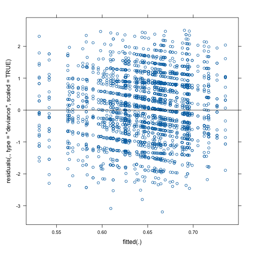
In this case the plot of residuals versus fitted values looks much better than in the binary case, since with more trials the values are closer to normal.
plot(
  galamm_mod_trials,
  form = residuals(., type = "deviance", scaled = TRUE) ~ fitted(.),
  abline = c(0, 0)
  )
Model with Poisson Distributed Responses
To illustrate the model for counts, we consider an example from Chapter 11.3 in Skrondal and Rabe-Hesketh (2004). The model does not contain factor loadings, but we use it to demonstrate how to fit GLMMs with Poisson distributed responses.
count_mod <- galamm(
  formula = y ~ lbas * treat + lage + v4 + (1 | subj),
  data = epilep,
  family = poisson
)
We can look at the summary output.
summary(count_mod)
#> GALAMM fit by maximum marginal likelihood.
#> Formula: y ~ lbas * treat + lage + v4 + (1 | subj)
#>    Data: epilep
#>
#>      AIC      BIC   logLik deviance df.resid
#>   1344.7   1369.0   -665.4    407.0      229
#>
#> Scaled residuals:
#>     Min      1Q  Median      3Q     Max
#> -3.1918 -0.8456 -0.0917  0.5839  6.6303
#>
#> Random effects:
#>  Groups Name        Variance Std.Dev.
#>  subj   (Intercept) 0.2516   0.5016
#> Number of obs: 236, groups:  subj, 59
#>
#> Fixed effects:
#>             Estimate Std. Error z value  Pr(>|z|)
#> (Intercept)   1.7936    0.10468  17.134 8.230e-66
#> lbas          0.8845    0.13096   6.754 1.436e-11
#> treat        -0.3350    0.14775  -2.267 2.339e-02
#> lage          0.4846    0.34658   1.398 1.621e-01
#> v4           -0.1611    0.05458  -2.952 3.161e-03
#> lbas:treat    0.3384    0.20293   1.668 9.541e-02
In this case there are no factor loadings to return:
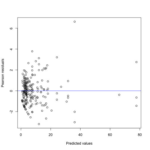
factor_loadings(count_mod)We can again look at a diagnostic plot.

We can also plot the residuals per subject:

In this case we can confirm that the galamm function is
correctly implemented by comparing it to the output of
lme4::glmer. For a model like this, it would also be best
to use lme4, but with factor structures or other
nonlinearities, lme4 no longer provides the flexibility we
need.
library(lme4)
#> Loading required package: Matrix
count_mod_lme4 <- glmer(
  formula = y ~ lbas * treat + lage + v4 + (1 | subj),
  data = epilep,
  family = poisson
)
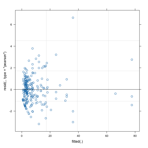
We can confirm that the diagnostic plot has the same values as for galamm:
plot(count_mod_lme4)
And we can do the same for the summary output.
summary(count_mod_lme4)
#> Generalized linear mixed model fit by maximum likelihood (Laplace Approximation) ['glmerMod']
#>  Family: poisson  ( log )
#> Formula: y ~ lbas * treat + lage + v4 + (1 | subj)
#>    Data: epilep
#>
#>       AIC       BIC    logLik -2*log(L)  df.resid
#>    1344.7    1369.0    -665.4    1330.7       229
#>
#> Scaled residuals:
#>     Min      1Q  Median      3Q     Max
#> -3.1918 -0.8456 -0.0918  0.5837  6.6303
#>
#> Random effects:
#>  Groups Name        Variance Std.Dev.
#>  subj   (Intercept) 0.2515   0.5015
#> Number of obs: 236, groups:  subj, 59
#>
#> Fixed effects:
#>             Estimate Std. Error z value Pr(>|z|)
#> (Intercept)   1.7937     0.1045  17.165  < 2e-16 ***
#> lbas          0.8844     0.1308   6.764 1.34e-11 ***
#> treat        -0.3349     0.1474  -2.272  0.02311 *
#> lage          0.4845     0.3458   1.401  0.16121
#> v4           -0.1611     0.0543  -2.966  0.00301 **
#> lbas:treat    0.3382     0.2025   1.671  0.09479 .
#> ---
#> Signif. codes:  0 '***' 0.001 '**' 0.01 '*' 0.05 '.' 0.1 ' ' 1
#>
#> Correlation of Fixed Effects:
#>            (Intr) lbas   treat  lage   v4
#> lbas       -0.035
#> treat      -0.708  0.024
#> lage       -0.092 -0.037  0.099
#> v4          0.015  0.000  0.000  0.000
#> lbas:treat  0.001 -0.654 -0.087  0.252  0.000
You might note that the deviance in the summary output of the model fitted by lme4 is different from the deviance of the model fitted by galamm. This is because in the summary output, lme4 shows the deviance as minus two times the log likelihood. In contrast, calling the deviance function on a model object fitted by glmer gives the same output as galamm.
deviance(count_mod_lme4)
#> [1] 407.0092
For details on deviance calculation in lme4, see
help(deviance.merMod, "lme4").