Interactions Between Latent and Observed Covariates
Source:vignettes/latent_observed_interaction.Rmd
latent_observed_interaction.RmdThis vignette describes how galamm can be used to model
interactions between latent and observed variables. The models described
here can be considered extensions of the covariate measurement error
model described in the vignette
on mixed response types, by allowing the latent variables to
interaction with observed variables.
Linear Mixed Model with Latent Covariates
For this example we use the simulated latent_covariates
dataset, of which the first six rows are displayed below:
head(latent_covariates)
#>   id         type         x            y response
#> 1  1 measurement1 0.2655087 -0.530999307        0
#> 2  1 measurement2 0.2655087 -0.911206495        0
#> 3  1     response 0.2655087  0.483055528        1
#> 4  2 measurement1 0.3721239  0.003752663        0
#> 5  2 measurement2 0.3721239  0.220165165        0
#> 6  2     response 0.3721239  0.327782922        1
Model Formulation
The response variable y contains both measurements of a
latent variable and measurements of the response that we actually are
interested in modeling, and the type variable distinguishes
these responses. In this case we have complete observations for each
subject ID, and for a given ID, the measurement model can be written as
follows:
In this equation is a vector of intercepts, is a latent variable, the loading of the latent variable onto the first measurement is fixed to 1 for identifiability, is the loading of the latent variable onto the second measurement , is the main effect of the latent variable on the response of interest , is the effect of the observed covariate on , and is the interaction effect of and on . We assume that the residuals are independently and identically normally distributed; this assumption is valid in this simulated case, but note that since the response is qualitatively different from the measurements and , this assumption will in general not hold, and a heteroscedastic measurement model should be used, or a model with mixed response types. For a more detailed explanation of this way of formulating latent variable models in matrix form we refer to the first four pages of Rockwood and Jeon (2019).
The structural model is simply , where is its variance.
Model Without Interaction
It can be instructive to start by considering a model in which we fix . This type of model would be estimated with the following code:
lambda <- matrix(c(1, NA, NA), ncol = 1)

mod0 <- galamm(
  formula = y ~ type + x:response + (0 + loading | id),
  data = latent_covariates,
  load_var = "type",
  lambda = lambda,
  factor = "loading"
)
In the data generating simulations, the true values were , and . The former two are very well recovered, but the latter is too positive, which is likely due to us omitting the interaction , whose true value was 0.2.
summary(mod0)
#> GALAMM fit by maximum marginal likelihood.
#> Formula: y ~ type + x:response + (0 + loading | id)
#>    Data: latent_covariates
#>
#>      AIC      BIC   logLik deviance df.resid
#>    197.5    232.7    -90.8    181.5      592
#>
#> Scaled residuals:
#>      Min       1Q   Median       3Q      Max
#> -2.92130 -0.52315 -0.01058  0.52532  3.01104
#>
#> Lambda:
#>         loading       SE
#> lambda1  1.0000        .
#> lambda2  1.3033 0.013687
#> lambda3 -0.2063 0.008515
#>
#> Random effects:
#>  Groups   Name    Variance Std.Dev.
#>  id       loading 0.98112  0.9905
#>  Residual         0.01357  0.1165
#> Number of obs: 600, groups:  id, 200
#>
#> Fixed effects:
#>                   Estimate Std. Error  t value  Pr(>|t|)
#> (Intercept)      -0.010588    0.07052 -0.15014 8.807e-01
#> typemeasurement2 -0.002173    0.02423 -0.08968 9.285e-01
#> typeresponse      0.029353    0.08678  0.33826 7.352e-01
#> x:response        0.470444    0.03093 15.20943 3.062e-52
Linear Interaction Between Observed and Latent Covariates
The measurement model can be equivalently written as
This way of writing shows more explicitly which factor loadings are
connected with which observation. In order to fit this model with
galamm, we must provide formulas for the terms in the
loading matrix
We specify the factor interactions with a list, one for each row of
lambda:
factor_interactions <- list(~ 1, ~ 1, ~ x)This specifies that for the first two rows, there are no covariates,
but for the third row, we want a linear regression with
as covariate. Next, we specify the loading matrix
without the interaction parameter, i.e., we reuse the
lambda object that was specified for mod0
above. This lets us fit the model as follows:
mod <- galamm(
  formula = y ~ type + x:response + (0 + loading | id),
  data = latent_covariates,
  load_var = "type",
  lambda = lambda,
  factor = "loading",
  factor_interactions = factor_interactions
)
A model comparison shows overwhelming evidence in favor of this model, which is not surprising since this is how the data were simulated.
anova(mod, mod0)
#> Data: latent_covariates
#> Models:
#> mod0: y ~ type + x:response + (0 + loading | id)
#> mod: y ~ type + x:response + (0 + loading | id)
#>      npar    AIC    BIC  logLik deviance Chisq Df Pr(>Chisq)
#> mod0    8 197.52 232.70 -90.761   120.31
#> mod     9 138.31 177.88 -60.155   120.31 61.21  1  5.129e-15 ***
#> ---
#> Signif. codes:  0 '***' 0.001 '**' 0.01 '*' 0.05 '.' 0.1 ' ' 1
The summary also shows that the bias in has basically disappeared, as it is up to -0.318 from -0.195, with the true value being -0.3. The interaction is estimated at 0.233, which is also very close to the true value 0.2. It should of course be noted here that the noise level in this simulated dataset was set unrealistically low, to let us confirm that the implementation itself is correct.
summary(mod)
#> GALAMM fit by maximum marginal likelihood.
#> Formula: y ~ type + x:response + (0 + loading | id)
#>    Data: latent_covariates
#>
#>      AIC      BIC   logLik deviance df.resid
#>    138.3    177.9    -60.2    120.3      591
#>
#> Scaled residuals:
#>     Min      1Q  Median      3Q     Max
#> -2.2033 -0.5251 -0.0273  0.5146  3.5029
#>
#> Lambda:
#>           loading      SE
#> lambda1    1.0000       .
#> lambda2    1.3034 0.01268
#> lambda3   -0.3183 0.01604
#> lambda4_x  0.2331 0.02873
#>
#> Random effects:
#>  Groups   Name    Variance Std.Dev.
#>  id       loading 0.98175  0.9908
#>  Residual         0.01164  0.1079
#> Number of obs: 600, groups:  id, 200
#>
#> Fixed effects:
#>                   Estimate Std. Error  t value  Pr(>|t|)
#> (Intercept)      -0.010589    0.07048 -0.15024 8.806e-01
#> typemeasurement2 -0.002173    0.02384 -0.09116 9.274e-01
#> typeresponse      0.034005    0.09417  0.36109 7.180e-01
#> x:response        0.462507    0.03300 14.01556 1.252e-44
Interaction Between Latent Covariate and a Quadratic Term
We can also try to add interactions between the
and
.
We first update the formula in factor_interactions:
Then we fit the model as before:
mod2 <- galamm(
  formula = y ~ type + x:response + (0 + loading | id),
  data = latent_covariates,
  load_var = "type",
  lambda = lambda,
  factor = "loading",
  factor_interactions = factor_interactions
)
As can be seen, the coefficient for this squared interaction is not significantly different from zero.
summary(mod2)
#> GALAMM fit by maximum marginal likelihood.
#> Formula: y ~ type + x:response + (0 + loading | id)
#>    Data: latent_covariates
#>
#>      AIC      BIC   logLik deviance df.resid
#>    140.3    184.2    -60.1    120.3      590
#>
#> Scaled residuals:
#>     Min      1Q  Median      3Q     Max
#> -2.2012 -0.5212 -0.0228  0.5173  3.4968
#>
#> Lambda:
#>                 loading      SE
#> lambda1         1.00000       .
#> lambda2         1.30340 0.01267
#> lambda3        -0.31418 0.02446
#> lambda4_x       0.20906 0.11252
#> lambda5_I(x^2)  0.02453 0.11097
#>
#> Random effects:
#>  Groups   Name    Variance Std.Dev.
#>  id       loading 0.98175  0.9908
#>  Residual         0.01164  0.1079
#> Number of obs: 600, groups:  id, 200
#>
#> Fixed effects:
#>                   Estimate Std. Error  t value  Pr(>|t|)
#> (Intercept)      -0.009919    0.07054 -0.14062 8.882e-01
#> typemeasurement2 -0.001969    0.02385 -0.08256 9.342e-01
#> typeresponse      0.033289    0.09426  0.35316 7.240e-01
#> x:response        0.462228    0.03305 13.98397 1.953e-44
Models with Additional Random Effects
It is also straightforward to include additional random effects in
models containing interactions between latent and observed covariates.
The dataset latent_covariates_long is similar to
latent_covariates that was used above, but it has six
repeated measurements of the response for each subject. The first ten
rows of the dataset are shown below.
head(latent_covariates_long, 10)
#>    id         type         x            y response
#> 1   1 measurement1 0.2655087 -0.530999307        0
#> 2   1 measurement2 0.2655087 -0.911206495        0
#> 3   1     response 0.2655087  0.250414575        1
#> 4   1     response 0.2655087  0.702355328        1
#> 5   2 measurement1 0.3721239  0.003752663        0
#> 6   2 measurement2 0.3721239  0.220165165        0
#> 7   2     response 0.3721239  0.337374818        1
#> 8   2     response 0.3721239  0.315766396        1
#> 9   3 measurement1 0.5728534 -0.902625075        0
#> 10  3 measurement2 0.5728534 -1.127476052        0
For these data we add a random intercept for the response terms, in addition to the terms that were used above. We start by resetting the interaction models to a linear term:
factor_interactions <- list(~ 1, ~ 1, ~ x)Next we fit the model using galamm. The difference to
notice here is that we added (0 + response | id) to the
formula. This implies that for observations that are responses, for
which response = 1, there should be a random intercept per
subject.
mod <- galamm(
  formula = y ~ type + x:response + (0 + loading | id) + (0 + response | id),
  data = latent_covariates_long,
  load_var = "type",
  lambda = lambda,
  factor = "loading",
  factor_interactions = factor_interactions
)
From the summary, we see that also in this case the factor loadings are very well recovered.
summary(mod)
#> GALAMM fit by maximum marginal likelihood.
#> Formula: y ~ type + x:response + (0 + loading | id) + (0 + response |      id)
#>    Data: latent_covariates_long
#>
#>      AIC      BIC   logLik deviance df.resid
#>    150.6    197.5    -65.3    130.6      790
#>
#> Scaled residuals:
#>     Min      1Q  Median      3Q     Max
#> -3.3804 -0.5291 -0.0199  0.5126  3.5849
#>
#> Lambda:
#>           loading      SE
#> lambda1    1.0000       .
#> lambda2    1.3036 0.01672
#> lambda3   -0.3279 0.01539
#> lambda4_x  0.2415 0.02730
#>
#> Random effects:
#>  Groups   Name     Variance Std.Dev.
#>  id       loading  0.97824  0.9891
#>  id.1     response 0.00000  0.0000
#>  Residual          0.02018  0.1420
#> Number of obs: 800, groups:  id, 200
#>
#> Fixed effects:
#>                   Estimate Std. Error  t value  Pr(>|t|)
#> (Intercept)      -0.010585    0.07065 -0.14981 8.809e-01
#> typemeasurement2 -0.002171    0.02555 -0.08498 9.323e-01
#> typeresponse      0.033712    0.09473  0.35590 7.219e-01
#> x:response        0.474623    0.03178 14.93242 2.028e-50
Model with Smooth Terms
We can also include smooth terms in models containing interactions
between latent and observed variables. In this example, we replace the
linear term x:response with a smooth term
s(x, by = response). Since this smooth term also includes
the main effect of response, which corresponds to an
intercept for the response observations, we must remove the
type term and instead insert two dummy variables, one for
each measurement. We first create these dummy variables:
dat <- latent_covariates
dat$m1 <- as.numeric(dat$type == "measurement1")
dat$m2 <- as.numeric(dat$type == "measurement2")
We then fit the model:
mod <- galamm(
  formula = y ~ 0 + m1 + m2 + s(x, by = response) + (0 + loading | id),
  data = dat,
  load_var = "type",
  lambda = lambda,
  factor = "loading",
  factor_interactions = factor_interactions
)
The summary output again suggest that the factor loadings are very well recovered.
summary(mod)
#> GALAMM fit by maximum marginal likelihood.
#> Formula: y ~ 0 + m1 + m2 + s(x, by = response) + (0 + loading | id)
#>    Data: dat
#>
#>      AIC      BIC   logLik deviance df.resid
#>    140.3    184.3    -60.2    120.3      590
#>
#> Scaled residuals:
#>     Min      1Q  Median      3Q     Max
#> -2.2032 -0.5251 -0.0273  0.5146  3.5029
#>
#> Lambda:
#>           loading      SE
#> lambda1    1.0000       .
#> lambda2    1.3034 0.01268
#> lambda3   -0.3183 0.01604
#> lambda4_x  0.2331 0.02873
#>
#> Random effects:
#>  Groups   Name          Variance Std.Dev.
#>  id       loading       0.98175  0.9908
#>  Xr       s(x):response 0.00000  0.0000
#>  Residual               0.01164  0.1079
#> Number of obs: 600, groups:  id, 200; Xr, 8
#>
#> Fixed effects:
#>                  Estimate Std. Error t value  Pr(>|t|)
#> m1               -0.01059   0.070477 -0.1503 8.805e-01
#> m2               -0.01276   0.091638 -0.1393 8.892e-01
#> s(x):responseFx1  0.12412   0.008856 14.0155 1.252e-44
#> s(x):responseFx2  0.26284   0.015809 16.6255 4.558e-62
#>
#> Approximate significance of smooth terms:
#>               edf Ref.df     F p-value
#> s(x):response   2      2 417.2  <2e-16
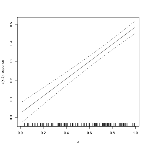
We can also plot the smooth term, which is linear. That is, in this
case the smooth term was not necessary. Not that we can also see this
from the zero variance estimate of the random effect named
s(x):response in the summary above, which mean that the
smoothing parameter for this term is infinite, and hence that the smooth
term is exactly linear.
plot_smooth(mod)
We can also make a diagnostic plot of residuals versus fitted value, and we see no clear trends.

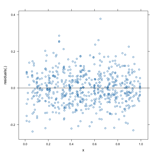
We can also plot the residuals against , and again we see no trends.
