Plot smooth terms for galamm fits

Plots smooth terms of a fitted galamm object. This function is a thin wrapper around mgcv::plot.gam (Wood 2017) .

Usage

# S3 method for galamm
plot_smooth(object, ...)

Arguments

object

Object of class galamm returned from galamm.

...

Other optional arguments, passed on to mgcv::plot.gam.

Value

A plot is displayed on the screen.

References

Wood SN (2017). Generalized Additive Models: An Introduction with R, 2 edition. Chapman and Hall/CRC.

See also

Other summary functions: anova.galamm(), plot.galamm(), print.summary.galamm(), summary.galamm()

Examples

# Generalized additive mixed model with factor structures -------------------

# The cognition dataset contains simulated measurements of three latent
# time-dependent processes, corresponding to individuals' abilities in
# cognitive domains. We focus here on the first domain, and take a single
# random timepoint per person:
dat <- subset(cognition, domain == 1)
dat <- split(dat, f = dat$id)
dat <- lapply(dat, function(x) x[x$timepoint %in% sample(x$timepoint, 1), ])
dat <- do.call(rbind, dat)
dat$item <- factor(dat$item)

# At each timepoint there are three items measuring ability in the cognitive
# domain. We fix the factor loading for the first measurement to one, and
# estimate the remaining two. This is specified in the loading matrix.
loading_matrix <- matrix(c(1, NA, NA), ncol = 1)

# We can now estimate the model.
mod <- galamm(
  formula = y ~ 0 + item + sl(x, factor = "loading") +
    (0 + loading | id),
  data = dat,
  load.var = "item",
  lambda = loading_matrix,
  factor = "loading"
)

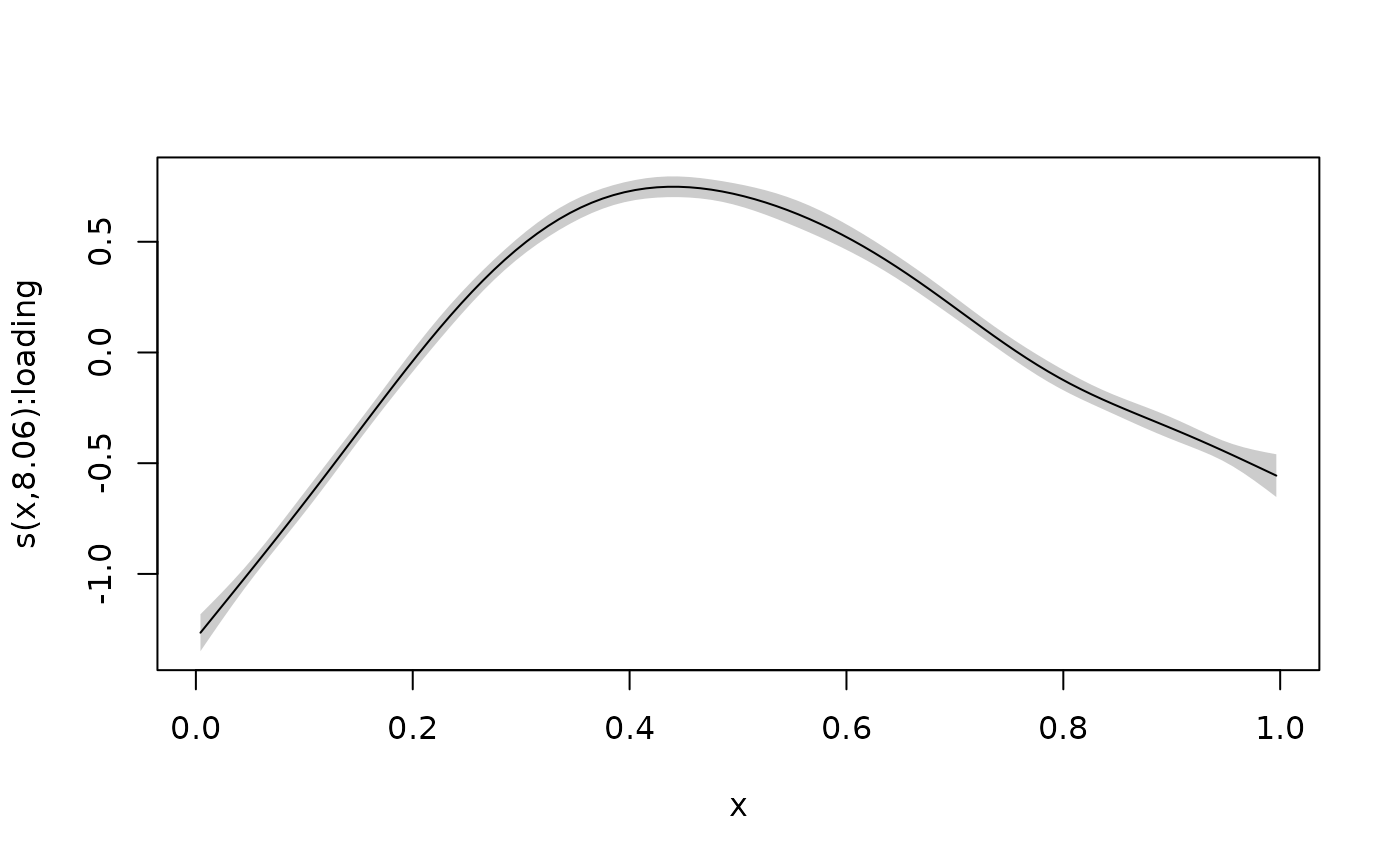
# We can plot the estimated smooth term
plot_smooth(mod, shade = TRUE)


# We can turn off the rug at the bottom
plot_smooth(mod, shade = TRUE, rug = FALSE)