This vignette describes how galamm can be used to
estimate linear mixed models with factor structures. Such models are an
instance of the generalized linear latent and mixed models (GLLAMM)
framework described by Rabe-Hesketh, Skrondal,
and Pickles (2004)
and Skrondal and Rabe-Hesketh (2004). The
R package PLmixed (Rockwood and Jeon
2019) estimates such models using a profile likelihood
algorithm initially proposed by Jeon and
Rabe-Hesketh (2012).
The models are also a special case of generalized additive latent and
mixed models (GALAMM), and in galamm these models are estimated using a
more direct algorithm described in Sørensen,
Fjell, and Walhovd (2023).
The examples used in this vignette come from the simulated datasets provided by PLmixed (Rockwood and Jeon 2019). The purpose of this vignette is to confirm that galamm gives the same results for these models, and to introduce the syntax. As will be clear if you run the code, galamm can often be considerably faster.
Crossed Random Effects Model with Persistence Parameters
This example comes from Section 3.1 in Jeon
and Rabe-Hesketh (2012),
whose model was again based on McCaffrey et al.
(2004).
The dataset KYPSsim comes from PLmixed and is a
simulated version of the Korea Youth Panel Survey (KYPS) data.
head(KYPSsim)
#>   mid hid sid time   esteem
#> 1   1   1   1    1 2.759234
#> 2   1   1   1    2 2.980368
#> 3   1   1   1    3 3.130784
#> 4   1   1   1    4 3.310306
#> 5   2   1   2    1 2.924520
#> 6   2   1   2    2 2.997440
Student self esteem (variable esteem) was assessed at
four timepoints, the first two while the student attended middle school,
and the second two while the student attended high school. The variables
mid and hid represent the middle school and
high school which a given student attended, and sid is the
student identifier. The variable time indicates the given
timepoint.
We will use a discrete time model, and hence convert the time variable to a factor.
Since students attending a given middle school not necessarily attend the same high school, we have a model with crossed random effects. We use the model of Jeon and Rabe-Hesketh (2012), whose measurement part can be formulated as
where is a vector whose th element equals one and all other elements equal zero. is an intercept, and , , and are the effects of timepoints 2, 3, and 4. and are the “teacher effects” of middle school and high school , respectively, is the latent level for student , and is a residual term. and are factor loadings (called “persistence parameters” by McCaffrey et al. (2004) and Jeon and Rabe-Hesketh (2012)) specifying how the teacher effects for middle school and high school impact the self esteem measurement. Since students attend high school after middle school, the measurements of self esteem in middle school are assumed not to be affected by high school, and hence the first two elements of are set to zero. The first nonzero element is set to zero for identifiability, so we have . Conversely, we allow for middle school to have an effect of measurements in high school, so , with the first element set to zero for identifiability. The residuals are assumed normally distributed, .
Written out for each of the four timepoints, the model becomes
The structural model is simply
where denotes a trivariate normal distribution with mean and covariance .
In order to fit the model with galamm, we use syntax similar to
PLmixed, and start by defining the loading matrix. The first column
contains
and the second column contains
.
Numerical values in this matrix means that the entry is fixed to the
given value, whereas NA means that the value is unknown,
and should be estimated.
(loading_matrix <- rbind(
  c(1, 0),
  c(NA, 0),
  c(NA, 1),
  c(NA, NA)
))
#>      [,1] [,2]
#> [1,]    1    0
#> [2,]   NA    0
#> [3,]   NA    1
#> [4,]   NA   NA
We connect the loading matrix to variables in the dataframe with the following factors.
factors <- c("ms", "hs")Finally, we define the loading variable. This is a variable
connecting rows of the dataframe to rows of the loading matrices. In
this case, for each value of time, the corresponding row of
the loading matrix should be multiplied by the latent variables
and
,
so we set it as follows:
load_var <- "time"The model formula is specified as
form <- esteem ~ time + (0 + ms | mid) + (0 + hs | hid) + (1 | sid)We use lme4 syntax for random effects. For example, the term
(0 + ms | mid) corresponds to
,
where | mid specifies that
should have a unique value for each unique mid. Since
"ms" can be found in the factors defined
above, this term should be treated specially, by making sure that the
latent variable is multiplied by the factor loading corresponding to
"ms" for each particular row. In contrast, the latent
variable for students
is a simple random intercept, and hence the term (1 | sid)
suffices.
We fit the model using galamm with the following
call.
mod <- galamm(
  formula = form,
  data = KYPSsim,
  factor = factors,
  load_var = load_var,
  lambda = loading_matrix
)
The model could be fit with PLmixed using the following
call, which differs from the call to galamm in that
factor and lambda must be put inside lists.
The reader is encouraged to try, and confirm that the results are
essentially equivalent, but we won’t run it in this vignette as it takes
5-10 minutes.
kyps_plmixed <- PLmixed(
  formula = form,
  data = KYPSsim,
  factor = list(factors),
  load_var = load_var,
  lambda = list(loading_matrix)
)
Using galamm’s summary method, we can study the model output.
summary(mod)
#> GALAMM fit by maximum marginal likelihood.
#> Formula: form
#>    Data: KYPSsim
#>
#>      AIC      BIC   logLik deviance df.resid
#>  19388.0  19476.2  -9682.0  19364.0    11482
#>
#> Scaled residuals:
#>     Min      1Q  Median      3Q     Max
#> -3.7952 -0.5945  0.0028  0.6049  3.5753
#>
#> Lambda:
#>              ms     SE    hs    SE
#> lambda1 1.00000      .     .     .
#> lambda2 0.87509 0.1421     .     .
#> lambda3 0.04432 0.1496 1.000     .
#> lambda4 0.02094 0.1543 1.502 0.504
#>
#> Random effects:
#>  Groups   Name        Variance Std.Dev.
#>  sid      (Intercept) 0.151749 0.38955
#>  hid      hs          0.005253 0.07248
#>  mid      ms          0.010695 0.10342
#>  Residual             0.222511 0.47171
#> Number of obs: 11494, groups:  sid, 2924; hid, 860; mid, 104
#>
#> Fixed effects:
#>             Estimate Std. Error t value  Pr(>|t|)
#> (Intercept)   3.1479    0.01524 206.619 0.000e+00
#> time2         0.1184    0.01253   9.451 3.361e-21
#> time3         0.1534    0.01607   9.547 1.339e-21
#> time4         0.1924    0.01675  11.489 1.496e-30
We can look at the factor loadings specifically using the
factor_loadings function. Perhaps not surprisingly, middle
school teacher effects have a low impact on self esteem while the
student attends high school, as can be seen by the last two rows of the
“ms” column being very close to zero.
factor_loadings(mod)
#>                 ms        SE       hs        SE
#> lambda1 1.00000000        NA 0.000000        NA
#> lambda2 0.87509307 0.1421073 0.000000        NA
#> lambda3 0.04431739 0.1495679 1.000000        NA
#> lambda4 0.02093662 0.1542824 1.501574 0.5040218
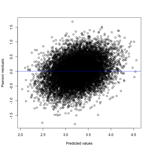
A diagnostic plot of residuals versus predicted values also looks acceptable, although there seems to be a slight upward trend.

We can also compare the estimated model to a model with constrained factor loadings. In particular, we could assume that the teacher effect in middle school has no effect on self esteem measured during high school, by setting the last two elements of to zero. We would then have the following loading matrix.
(loading_matrix_constr1 <- rbind(
  c(1, 0),
  c(NA, 0),
  c(0, 1),
  c(0, NA)
))
#>      [,1] [,2]
#> [1,]    1    0
#> [2,]   NA    0
#> [3,]    0    1
#> [4,]    0   NA
mod_constr1 <- galamm(
  formula = form,
  data = KYPSsim,
  factor = factors,
  load_var = load_var,
  lambda = loading_matrix_constr1
)
We could further assume that the factor loadings at timepoints 1 and 2 for middle school and at timepoints 3 and 4 for high schools are identical, which in practice would lead to a linear mixed model with no factors. One way of estimating this model is to define a new loading matrix:
(loading_matrix_constr2 <- rbind(
  c(1, 0),
  c(1, 0),
  c(0, 1),
  c(0, 1)
))
#>      [,1] [,2]
#> [1,]    1    0
#> [2,]    1    0
#> [3,]    0    1
#> [4,]    0    1
mod_constr2 <- galamm(
  formula = form,
  data = KYPSsim,
  factor = factors,
  load_var = load_var,
  lambda = loading_matrix_constr2
)
Equivalently, we could create dummy variables for the timepoints:
KYPSsim$time12 <- as.integer(KYPSsim$time %in% 1:2)
KYPSsim$time34 <- as.integer(KYPSsim$time %in% 3:4)
head(KYPSsim)
#>   mid hid sid time   esteem time12 time34
#> 1   1   1   1    1 2.759234      1      0
#> 2   1   1   1    2 2.980368      1      0
#> 3   1   1   1    3 3.130784      0      1
#> 4   1   1   1    4 3.310306      0      1
#> 5   2   1   2    1 2.924520      1      0
#> 6   2   1   2    2 2.997440      1      0
We this formulation, we don’t need to specify the
factor, load_var, and lambda
arguments.
mod_constr2b <- galamm(
  formula = esteem ~ time + (0 + time12 | mid) + (0 + time34 | hid) + (1 | sid),
  data = KYPSsim
)
We can compare all four models using the anova member
function. Reassuringly, the two ways of formulating the last model give
identical results. Furthermore, this simplest model seems to be
preferred over the two more complex models on this simulated
dataset.
anova(
  mod, mod_constr1, mod_constr2,
  mod_constr2b
)
#> Data: KYPSsim
#> Models:
#> mod_constr2: form
#> mod_constr2b: esteem ~ time + (0 + time12 | mid) + (0 + time34 | hid) + (1 |     sid)
#> mod_constr1: form
#> mod: form
#>              npar   AIC   BIC  logLik deviance   Chisq Df Pr(>Chisq)
#> mod_constr2     8 19394 19452 -9688.9    19364
#> mod_constr2b    8 19394 19452 -9688.9    19364  0.0000  0
#> mod_constr1    10 19397 19471 -9688.5    19364  0.6661  2   0.716735
#> mod            12 19388 19476 -9682.0    19364 13.1070  2   0.001425 **
#> ---
#> Signif. codes:  0 '***' 0.001 '**' 0.01 '*' 0.05 '.' 0.1 ' ' 1
Multi-Trait Multi-Rater Model
We next consider a model based on example 1 in Rockwood and Jeon (2019),
which uses the dataset JUDGEsim in PLmixed, which is
simulated to mimic the data used by Koch et al.
(2016). We
refer to Rockwood and Jeon (2019)
for all the details, and merely present the model and how to estimate it
using galamm. Note however that although the fit with
galamm is identical to that presented in Rockwood and Jeon (2019),
our estimated factor loadings appear to differ from those in the table
at the bottom of page 298 in Rockwood and Jeon
(2019),
due to an error in the way the matrix of factor loadings was presented
in PLmixed versions <= 0.1.6. This issue
has been fixed in PLmixed version 0.1.7
(Nicholas Rockwood, personal communication, August 2023).
The data contains ratings of two traits in students, and the traits are rated by both students and teachers.
Initially, we need to convert the item variable to a factor.
JUDGEsim$item <- factor(JUDGEsim$item)The first ten rows of the dataset are as follows:
head(JUDGEsim, 10)
#>    item method trait stu class tch response
#> 1     1      1     1   1     1   1 2.509475
#> 2     1      1     1   1     1   2 3.246730
#> 3     1      1     1   1     1   3 2.846695
#> 4     1      1     1   1     1   4 2.290954
#> 5     1      1     1   1     1   5 2.794368
#> 6     1      1     1   1     1   6 2.849511
#> 7     1      1     1   1     1   7 2.255039
#> 8     1      1     1   2     1   1 2.676437
#> 9     1      1     1   2     1   2 2.923184
#> 10    1      1     1   2     1   3 2.778979
The grouping factors in the data are class (variable
class), student (variable stu) and teacher
(variable tch). The teachers’ ratings of the first trait is
given by items 1-3, and the students’ rating of the same trait is given
by items 7-9. For the second trait, the items are 4-6 and 10-12,
respectively. Looking at the frequency table, we see that there are more
observations of items 1-6. This happens because a single teacher would
in general rate more than one student, whereas a single student would
only rate themselves.
table(JUDGEsim$item)
#>
#>    1    2    3    4    5    6    7    8    9   10   11   12
#> 7828 7828 7828 7828 7828 7828 1249 1249 1249 1249 1249 1249
In matrix-vector format, the measurement model is (equation 16 in Rockwood and Jeon (2019))
In brief, and are the teacher effects, and are teacher’s perception of the students on the trait, and are the students’ perception of themselves on the trait, and is the classroom effect. The factor loadings are the “regression coefficients” for regressing the observed items onto these latent traits. The subscripts , , and indicate teacher, student, and class, respectively.
The structural model is simply
where
and
We specify the loading matrix as follows. In comparison with the mathematical model formulation just above, note that we don’t need to add the last column of only ones, since this column contains no parameters to be estimated.
(loading_matrix <- rbind(
  c(1, 0, 1, 0, 0, 0),
  c(NA, 0, NA, 0, 0, 0),
  c(NA, 0, NA, 0, 0, 0),
  c(0, 1, 0, 1, 0, 0),
  c(0, NA, 0, NA, 0, 0),
  c(0, NA, 0, NA, 0, 0),
  c(0, 0, 0, 0, 1, 0),
  c(0, 0, 0, 0, NA, 0),
  c(0, 0, 0, 0, NA, 0),
  c(0, 0, 0, 0, 0, 1),
  c(0, 0, 0, 0, 0, NA),
  c(0, 0, 0, 0, 0, NA)
))
#>       [,1] [,2] [,3] [,4] [,5] [,6]
#>  [1,]    1    0    1    0    0    0
#>  [2,]   NA    0   NA    0    0    0
#>  [3,]   NA    0   NA    0    0    0
#>  [4,]    0    1    0    1    0    0
#>  [5,]    0   NA    0   NA    0    0
#>  [6,]    0   NA    0   NA    0    0
#>  [7,]    0    0    0    0    1    0
#>  [8,]    0    0    0    0   NA    0
#>  [9,]    0    0    0    0   NA    0
#> [10,]    0    0    0    0    0    1
#> [11,]    0    0    0    0    0   NA
#> [12,]    0    0    0    0    0   NA
Next, we specify the factors in the order they appear in the columns of the loading matrix. We can choose whichever names we like for the factors, except for names of existing variables in the dataset, but we must make sure they match the names used in the formula.
factors <- c(
  "teacher1", "teacher2", "trait1.t",
  "trait2.t", "trait1.s", "trait2.s"
)
The formula is defined as follows, where have have placed the terms in the same order as they appear in the mathematical model in matrix-vector form specified above.
form <- response ~ 0 + item + (0 + teacher1 + teacher2 | tch) +
  (0 + trait1.t + trait2.t + trait1.s + trait2.s | stu) +
  (1 | class)
Using PLmixed, we could have estimated the model as
follows, and doing it would confirm that the results are the same as
with galamm.
judge_plmixed <- PLmixed(
  formula = form,
  data = JUDGEsim,
  lambda = list(loading_matrix),
  load_var = "item",
  factor = list(factors)
)
We get identical results using galamm, and it takes less
than five minutes.
judge_galamm <- galamm(
  formula = form,
  data = JUDGEsim,
  lambda = loading_matrix,
  load_var = "item",
  factor = factors
)
summary(judge_galamm)
#> GALAMM fit by maximum marginal likelihood.
#> Formula: form
#>    Data: JUDGEsim
#>
#>      AIC      BIC   logLik deviance df.resid
#> 113184.6 113531.9 -56553.3 113106.6    54423
#>
#> Scaled residuals:
#>     Min      1Q  Median      3Q     Max
#> -3.8407 -0.6439  0.0017  0.6474  3.9799
#>
#> Lambda:
#>          teacher1      SE teacher2      SE trait1.t      SE trait2.t      SE trait1.s      SE trait2.s
#> lambda1    1.0000       .        .       .    1.000       .        .       .        .       .        .
#> lambda2    1.1278 0.03584        .       .    1.092 0.02172        .       .        .       .        .
#> lambda3    0.9986 0.03345        .       .    1.066 0.02144        .       .        .       .        .
#> lambda4         .       .   1.0000       .        .       .   1.0000       .        .       .        .
#> lambda5         .       .   0.9725 0.03036        .       .   1.0536 0.02576        .       .        .
#> lambda6         .       .   1.2191 0.03436        .       .   0.9581 0.02460        .       .        .
#> lambda7         .       .        .       .        .       .        .       .    1.000       .        .
#> lambda8         .       .        .       .        .       .        .       .    1.322 0.06109        .
#> lambda9         .       .        .       .        .       .        .       .    1.145 0.05633        .
#> lambda10        .       .        .       .        .       .        .       .        .       .    1.000
#> lambda11        .       .        .       .        .       .        .       .        .       .    0.874
#> lambda12        .       .        .       .        .       .        .       .        .       .    1.096
#>               SE
#> lambda1        .
#> lambda2        .
#> lambda3        .
#> lambda4        .
#> lambda5        .
#> lambda6        .
#> lambda7        .
#> lambda8        .
#> lambda9        .
#> lambda10       .
#> lambda11 0.04417
#> lambda12 0.04874
#>
#> Random effects:
#>  Groups   Name        Variance Std.Dev. Corr
#>  stu      trait1.t    0.24025  0.4902
#>           trait2.t    0.16872  0.4108   0.86
#>           trait1.s    0.29588  0.5439   0.46 0.40
#>           trait2.s    0.37690  0.6139   0.20 0.30 0.40
#>  tch      teacher1    0.09704  0.3115
#>           teacher2    0.11321  0.3365   0.44
#>  class    (Intercept) 0.00000  0.0000
#>  Residual             0.39044  0.6249
#> Number of obs: 54462, groups:  stu, 1249; tch, 390; class, 125
#>
#> Fixed effects:
#>        Estimate Std. Error t value Pr(>|t|)
#> item1     3.399    0.02270  149.72        0
#> item2     3.363    0.02502  134.42        0
#> item3     3.362    0.02329  144.38        0
#> item4     2.820    0.02226  126.65        0
#> item5     2.939    0.02225  132.08        0
#> item6     2.877    0.02512  114.53        0
#> item7     3.426    0.02344  146.16        0
#> item8     3.552    0.02696  131.77        0
#> item9     3.597    0.02496  144.11        0
#> item10    2.334    0.02479   94.17        0
#> item11    2.909    0.02330  124.83        0
#> item12    2.470    0.02599   95.07        0
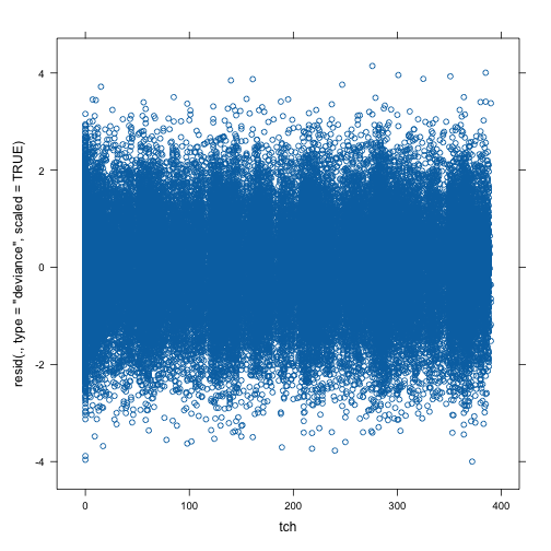
We can make various diagnostic plots. The one below plots scaled deviance residuals against teacher. It does not look like the residuals depend on teacher.

The quantile-quantile plot also looks very good (no surprise: these are simulated data).
qqmath(judge_galamm)
