Semiparametric Latent Variable Modeling • galamm

library(galamm)
library(gamm4)

This vignette describes how to use galamm to estimate latent variable models with smooth terms, or equivalently, generalized additive mixed models with factor structures. The examples are based on Section 4 and 5 in Sørensen, Fjell, and Walhovd (2023), but as we cannot share the data, we have instead simulated somewhat simpler datasets that will be used. We will gradually add complexity, starting with a simple generalized additive mixed model. Please refer to the introductory vignette for an overview of the statistical models.

Generalized Additive Mixed Models

We start by showing how galamm can be used to estimated generalized additive mixed models.

Gaussian Responses

The cognition dataset contains simulated data with measurements of abilities in three cognitive domains.

head(cognition)
#>   id domain          x timepoint item trials          y
#> 1  1      1 0.06475113         1   11      1 0.16788973
#> 2  1      1 0.06475113         1   12      1 0.08897838
#> 3  1      1 0.06475113         1   13      1 0.03162123
#> 4  1      1 0.15766278         2   11      1 0.46598362
#> 5  1      1 0.15766278         2   12      1 0.84564656
#> 6  1      1 0.15766278         2   13      1 0.20549872

For this first example, we focus only on the first item measured for the first domain.

dat <- subset(cognition, domain == 1 & item == "11")

Each subject in this dataset has been measured eight times, and we can plot the measurements as follows:

plot(dat$x, dat$y, type = "n", xlab = "x", ylab = "y")
for(i in unique(dat$id)) {
  dd <- dat[dat$id == i, ]
  lines(dd$x, dd$y, col = "gray")
}
points(dat$x, dat$y, pch = 20, lwd = .05)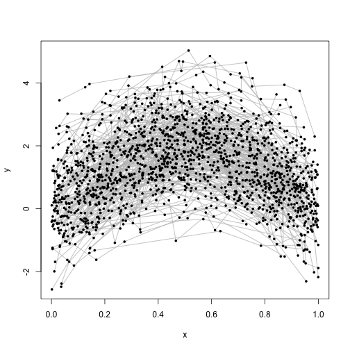

Plot of data for domain 1 and item 11.

We use a generalized additive mixed model with random intercepts per subject to estimate the function relating $x$ to $y$ . In terms of the model framework outlined in the introductory vignette, we model the $i$ th response from the $j$ th subject with

$y_{ij} = f(x_{ij}) + \eta_{j} + \epsilon_{ij}$

where $f(x_{ij})$ is a smooth function to be estimated, $\eta_{j} \sim N(0, \psi)$ is a random intercept, and $\epsilon_{ij} \sim N(0, \phi)$ is a residual term.

This model can be estimated using gamm4 as follows:

mod_gamm4 <- gamm4(y ~ s(x), random = ~ (1 | id), data = dat, REML = FALSE)

The package gamm4 uses lme4 to fit the underlying model, and the resulting model has two components. mod_gamm4$mer contains the mixed model representation, whereas in mod_gamm4$gam the fixed and random effects corresponding to spline coefficients have been converted into single smooth terms. We can look at the model summary for each:

summary(mod_gamm4$mer)
#> Linear mixed model fit by maximum likelihood  ['lmerMod']
#> 
#>      AIC      BIC   logLik deviance df.resid 
#>   3025.2   3052.1  -1507.6   3015.2     1595 
#> 
#> Scaled residuals: 
#>      Min       1Q   Median       3Q      Max 
#> -2.93755 -0.65215  0.00612  0.62654  3.14289 
#> 
#> Random effects:
#>  Groups   Name        Variance Std.Dev.
#>  id       (Intercept) 0.8551   0.9247  
#>  Xr       s(x)        2.0341   1.4262  
#>  Residual             0.2501   0.5001  
#> Number of obs: 1600, groups:  id, 200; Xr, 8
#> 
#> Fixed effects:
#>              Estimate Std. Error t value
#> X(Intercept)  1.26938    0.06657  19.067
#> Xs(x)Fx1     -0.15814    0.20156  -0.785
#> 
#> Correlation of Fixed Effects:
#>          X(Int)
#> Xs(x)Fx1 0.000
summary(mod_gamm4$gam)
#> 
#> Family: gaussian 
#> Link function: identity 
#> 
#> Formula:
#> y ~ s(x)
#> 
#> Parametric coefficients:
#>             Estimate Std. Error t value Pr(>|t|)    
#> (Intercept)  1.26938    0.06657   19.07   <2e-16 ***
#> ---
#> Signif. codes:  0 '***' 0.001 '**' 0.01 '*' 0.05 '.' 0.1 ' ' 1
#> 
#> Approximate significance of smooth terms:
#>        edf Ref.df     F p-value    
#> s(x) 6.681  6.681 324.9  <2e-16 ***
#> ---
#> Signif. codes:  0 '***' 0.001 '**' 0.01 '*' 0.05 '.' 0.1 ' ' 1
#> 
#> R-sq.(adj) =  0.253   
#> lmer.REML = 3015.2  Scale est. = 0.25012   n = 1600

We can also plot the estimated smooth term:

plot(mod_gamm4$gam)

Smooth term estimated by gamm4.

In contrast, invoking the plot function on the mixed model part gives us a diagnostic plot.

plot(mod_gamm4$mer)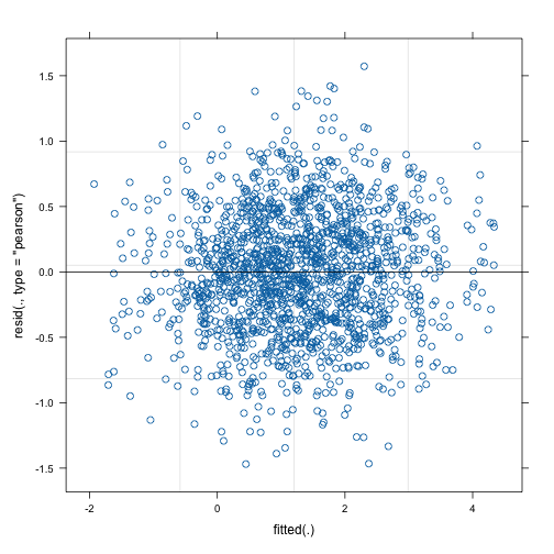

Diagnostic plot for gamm4 model.

With galamm we use similar argument, but the random specification is now part of the model formula.

mod <- galamm(y ~ s(x) + (1 | id), data = dat)

As opposed to gamm4, galamm gives a single summary. As can be seen, smooth terms are both reported as random effects, and in a separate line under the header “Approximate significance of smooth terms:”. Reassuringly, the results from fitting the model with gamm4 and with galamm are essentially equally, even though they use somewhat different computational algorithms.

summary(mod)
#> GALAMM fit by maximum marginal likelihood.
#> Formula: y ~ s(x) + (1 | id)
#>    Data: dat
#> 
#>      AIC      BIC   logLik deviance df.resid 
#>   3025.2   3052.1  -1507.6   3015.2     1595 
#> 
#> Scaled residuals: 
#>      Min       1Q   Median       3Q      Max 
#> -2.93755 -0.65215  0.00612  0.62654  3.14290 
#> 
#> Random effects:
#>  Groups   Name        Variance Std.Dev.
#>  id       (Intercept) 0.8551   0.9247  
#>  Xr       s(x)        2.0346   1.4264  
#>  Residual             0.2501   0.5001  
#> Number of obs: 1600, groups:  id, 200; Xr, 8
#> 
#> Fixed effects:
#>             Estimate Std. Error t value  Pr(>|t|)
#> (Intercept)   1.2694    0.06657 19.0672 4.731e-81
#> s(x)Fx1      -0.1582    0.20236 -0.7818 4.343e-01
#> 
#> Approximate significance of smooth terms:
#>        edf Ref.df     F p-value
#> s(x) 6.681  6.681 324.9  <2e-16

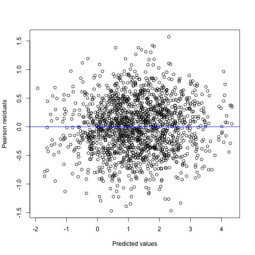
The plot function now gives us a diagnostic plot, which by inspection can be seen to be almost identical to the plot produced from the mixed model part of the gamm4 model.

plot(mod)

Diagnostic plot for model fitted with galamm.

In order to plot the smooth term, we use plot_smooth.

plot_smooth(mod)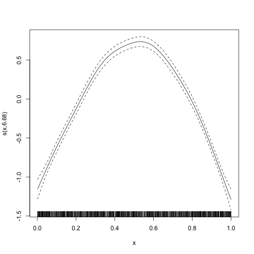

Smooth term estimated with galamm.

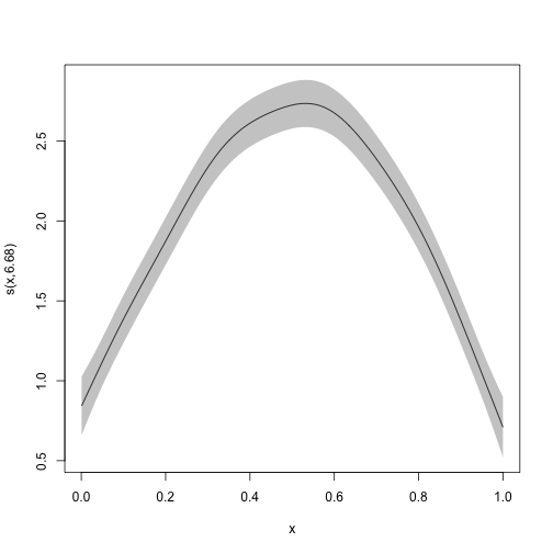
The plot_smooth function is a thin wrapper around the plot.gam function provided by the mgcv package (Wood 2017). This means that the arguments used by plot.gam can be used also here, as see with the examples below:

plot_smooth(mod,
  shade = TRUE, rug = FALSE, seWithMean = TRUE,
  shift = +2
)

Alternative ways of visualizing the smooth term.

plot_smooth(mod, se = FALSE)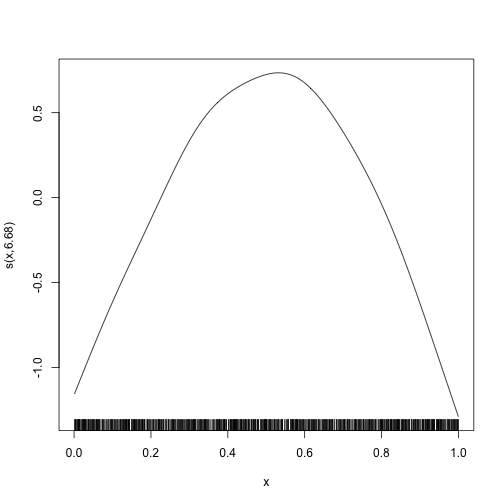

Alternative ways of visualizing the smooth term.

Binomial Responses

In the cognition dataset, the responses relating to domain 2 are binomially distributed. We will use the first trial to illustrate how such data can be modeled.

dat <- subset(cognition, domain == 2 & item == "21")

Again we can fit this model using gamm4.

mod_gamm4 <- gamm4(y ~ s(x),
  random = ~ (1 | id),
  data = dat, family = binomial
)

We can look at the summary output as before.

summary(mod_gamm4$mer)
#> Generalized linear mixed model fit by maximum likelihood (Laplace Approximation) ['glmerMod']
#>  Family: binomial  ( logit )
#> 
#>      AIC      BIC   logLik deviance df.resid 
#>    983.7   1005.2   -487.8    975.7     1596 
#> 
#> Scaled residuals: 
#>     Min      1Q  Median      3Q     Max 
#> -8.2548  0.0786  0.1946  0.4248  0.8213 
#> 
#> Random effects:
#>  Groups Name        Variance Std.Dev.
#>  id     (Intercept) 0.2306   0.4802  
#>  Xr     s(x)        0.9695   0.9846  
#> Number of obs: 1600, groups:  id, 200; Xr, 8
#> 
#> Fixed effects:
#>              Estimate Std. Error z value Pr(>|z|)    
#> X(Intercept)   2.8115     0.2034  13.825  < 2e-16 ***
#> Xs(x)Fx1      -1.4110     0.4242  -3.327 0.000879 ***
#> ---
#> Signif. codes:  0 '***' 0.001 '**' 0.01 '*' 0.05 '.' 0.1 ' ' 1
#> 
#> Correlation of Fixed Effects:
#>          X(Int)
#> Xs(x)Fx1 -0.440
summary(mod_gamm4$gam)
#> 
#> Family: binomial 
#> Link function: logit 
#> 
#> Formula:
#> y ~ s(x)
#> 
#> Parametric coefficients:
#>             Estimate Std. Error z value Pr(>|z|)    
#> (Intercept)   2.8115     0.1662   16.91   <2e-16 ***
#> ---
#> Signif. codes:  0 '***' 0.001 '**' 0.01 '*' 0.05 '.' 0.1 ' ' 1
#> 
#> Approximate significance of smooth terms:
#>       edf Ref.df Chi.sq p-value    
#> s(x) 2.14   2.14  113.9  <2e-16 ***
#> ---
#> Signif. codes:  0 '***' 0.001 '**' 0.01 '*' 0.05 '.' 0.1 ' ' 1
#> 
#> R-sq.(adj) =  0.116   
#> glmer.ML = 908.96  Scale est. = 1         n = 1600

And we can plot the smooth term. The diagnostic plot is not very useful in the binomial case, so we omit it.

plot(mod_gamm4$gam)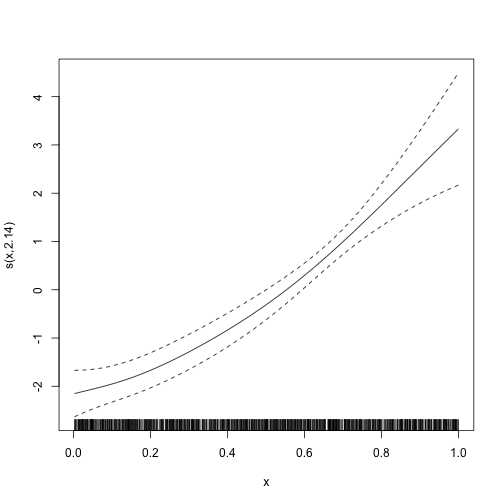

Smooth term estimated by gamm4.

Again the galamm syntax is similar, but it puts the random effect specification into the model formula.

mod <- galamm(y ~ s(x) + (1 | id), data = dat, family = binomial)

The estimates are very similar, although not identical. The difference in deviance is due to differences in the way deviance is defined. The call deviance(mod_gamm4$mer) gives the same value as in the summary for the model fitted with galamm.

summary(mod)
#> GALAMM fit by maximum marginal likelihood.
#> Formula: y ~ s(x) + (1 | id)
#>    Data: dat
#> 
#>      AIC      BIC   logLik deviance df.resid 
#>    983.7   1005.2   -487.8    908.8     1596 
#> 
#> Scaled residuals: 
#>     Min      1Q  Median      3Q     Max 
#> -8.2237  0.0792  0.1947  0.4245  0.8226 
#> 
#> Random effects:
#>  Groups Name        Variance Std.Dev.
#>  id     (Intercept) 0.2316   0.4813  
#>  Xr     s(x)        0.9387   0.9688  
#> Number of obs: 1600, groups:  id, 200; Xr, 8
#> 
#> Fixed effects:
#>             Estimate Std. Error z value  Pr(>|z|)
#> (Intercept)    2.808     0.1956  14.354 9.989e-47
#> s(x)Fx1       -1.406     0.4134  -3.402 6.697e-04
#> 
#> Approximate significance of smooth terms:
#>        edf Ref.df Chi.sq p-value
#> s(x) 2.124  2.124    114  <2e-16

plot_smooth(mod)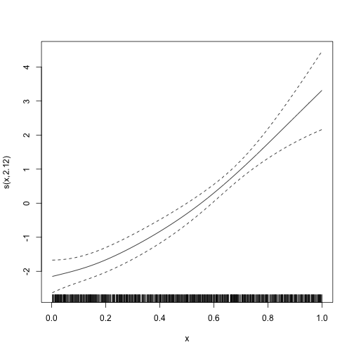

Smooth term estimated with galamm.

Generalized Additive Models with Factor Structures

We now add factor structures to the GAMMs. These are the types of models that neither gamm4 nor mgcv are able to estimate (at least without lots of manual hacking), and where galamm provides new functionality.

Gaussian Responses

To illustrate basic usage, we continue with the cognition data, but now use all items of cognitive domain 1. These are all conditionally normal distributed.

dat <- subset(cognition, domain == 1)
head(dat)
#>   id domain          x timepoint item trials          y
#> 1  1      1 0.06475113         1   11      1 0.16788973
#> 2  1      1 0.06475113         1   12      1 0.08897838
#> 3  1      1 0.06475113         1   13      1 0.03162123
#> 4  1      1 0.15766278         2   11      1 0.46598362
#> 5  1      1 0.15766278         2   12      1 0.84564656
#> 6  1      1 0.15766278         2   13      1 0.20549872

We now need a factor model to associate the underlying latent trait $\eta$ with the measurements $y_{i}$ :

$y_{i} = \beta_{i} + \lambda_{i} \eta + \epsilon_{i}$

In the structural model, we have a smooth term for the relationship between the latent trait and x, and we have random intercepts for a given timepoint within subject $\zeta^{(2)}$ , and for a given subject across timepoints $\zeta^{(3)}$ .

$\eta = h(x) + \zeta^{(2)} + \zeta^{(3)}.$

The reduced form of the model is

$y_{i} = \beta_{i} + \lambda_{i} \left\{ h(x) + \zeta^{(2)} + \zeta^{(3)} \right\} + \epsilon_{i}$

We will use a varying-coefficient term, where $h(x)$ is being interpreted as a regression coefficient for the effect of $\lambda_{i}$ on $y_{i}$ , and the regression term varies with $x$ . In contrast to Hastie and Tibshirani (1993) and other uses of varying-coefficient terms, however, in this case the predictor $\lambda_{i}$ is a model parameter. We have three items loading in $\eta$ and fix the first loading to 1 for identifiability, so the loading matrix is as follows:

(loading_matrix <- matrix(c(1, NA, NA), ncol = 1))
#>      [,1]
#> [1,]    1
#> [2,]   NA
#> [3,]   NA

We provide thin wrappers around the s() and t2() functions from mgcv to support factor loadings in smooth terms. The wrappers are named sl() and t2l() to avoid namespace conflicts with mgcv and gamm4, and the last letter “l” stands for “loading”. In this example, we set factor = "item" to specify that the loadings to be applied are identified by the “item” variable. Using mgcv’s by variable would also work in this particular case, i.e., replacing sl(x, factor = "loading") with s(x, by = loading). However, in most cases this would lead to identifiability issues due to the way varying-coefficient terms are set up by mgcv, so galamm provides an additional factor argument which alleviates most of these issues.

mod <- galamm(
  formula = y ~ 0 + item + sl(x, factor = "loading") +
    (0 + loading | id / timepoint),
  data = dat,
  load.var = "item",
  lambda = loading_matrix,
  factor = "loading"
)

We print the model summary below. In the data simulation, the factor loadings were set to 1, 1.4, and 0.3, respectively, and this is very well recovered. Furthermore, the ground truth standard deviation at the id level was 1, at the timepoint level it was 0.5, and the residual standard deviation was 0.1. The estimates are close to these values. Real data will typically not have this strong signal, but based on these results, there are no clear indications that the model is implemented incorrectly.

summary(mod)
#> GALAMM fit by maximum marginal likelihood.
#> Formula: y ~ 0 + item + sl(x, factor = "loading") + (0 + loading | id/timepoint)
#>    Data: dat
#> 
#>      AIC      BIC   logLik deviance df.resid 
#>   -918.2   -853.4    469.1   -938.2     4790 
#> 
#> Scaled residuals: 
#>    Min     1Q Median     3Q    Max 
#>  0.693 10.402 26.734 35.728 51.878 
#> 
#> Lambda:
#>         loading       SE
#> lambda1  1.0000        .
#> lambda2  1.3973 0.003531
#> lambda3  0.3009 0.002146
#> 
#> Random effects:
#>  Groups       Name         Variance Std.Dev.
#>  timepoint:id loading      0.236886 0.48671 
#>  id           loading      0.857051 0.92577 
#>  Xr           s(x):loading 2.030613 1.42500 
#>  Residual                  0.009932 0.09966 
#> Number of obs: 4800, groups:  timepoint:id, 1600; id, 200; Xr, 8
#> 
#> Fixed effects:
#>                 Estimate Std. Error t value  Pr(>|t|)
#> item11            1.2694    0.06663 19.0513 6.412e-81
#> item12            1.7788    0.09307 19.1128 1.977e-81
#> item13            0.3797    0.02019 18.8077 6.531e-79
#> s(x):loadingFx1  -0.1496    0.19977 -0.7488 4.540e-01
#> 
#> Approximate significance of smooth terms:
#>                edf Ref.df    F p-value
#> s(x):loading 8.719  8.719 4469  <2e-16

We also plot the smooth term. Since we had a very large amount of data, there is essentially no uncertainty about the estimate.

plot_smooth(mod)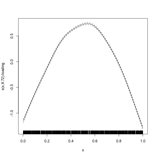

Smooth term for GAMM with factor structure.

Binomial Responses

We can now move on to the part of the cognition data that is conditionally binomially distributed. We consider domain 2, where each response measures success or not in a single trial. In this case there are only two items, so we must change the lambda matrix accordingly. Other than that, and setting family = binomial, the model is the same as before.

dat <- subset(cognition, domain == 2)

mod <- galamm(
  formula = y ~ 0 + item + sl(x, factor = "loading") +
    (0 + loading | id / timepoint),
  data = dat,
  family = binomial,
  load.var = "item",
  lambda = matrix(c(1, NA), ncol = 1),
  factor = "loading"
)

The summary is shown below. The factor loading $\lambda_{2} = 2$ was used when simulating the data, and including the uncertainty, our estimate covers the true value well. Also note that the variation between individuals (group id) and the variation between timepoints within individuals (group timepoint:id) gets lumped together at the id level. The estimated variation at the timepoint:id level is zero. This is a well-known phenomenon when fitting mixed models, given book-length treatment in Hodges (2013). In this case, it is likely due to the fact that we only have two measurements at each timepoint, and also the fact that we use the Laplace approximation to integrate over the random effects, and this approximation may be inaccurate for binomial data with a low number of repeated observations (Joe 2008).

summary(mod)
#> GALAMM fit by maximum marginal likelihood.
#> Formula: y ~ 0 + item + sl(x, factor = "loading") + (0 + loading | id/timepoint)
#>    Data: dat
#> 
#>      AIC      BIC   logLik deviance df.resid 
#>   1495.5   1538.0   -740.8   1614.8     3193 
#> 
#> Scaled residuals: 
#>      Min       1Q   Median       3Q      Max 
#> -15.8546   0.0279   0.0780   0.1985   1.3948 
#> 
#> Lambda:
#>         loading     SE
#> lambda1   1.000      .
#> lambda2   2.202 0.3007
#> 
#> Random effects:
#>  Groups       Name         Variance Std.Dev.
#>  timepoint:id loading      0.0000   0.0000  
#>  id           loading      0.6222   0.7888  
#>  Xr           s(x):loading 1.5388   1.2405  
#> Number of obs: 3200, groups:  timepoint:id, 1600; id, 200; Xr, 8
#> 
#> Fixed effects:
#>                 Estimate Std. Error z value  Pr(>|z|)
#> item21             2.944     0.1903  15.473 5.249e-54
#> item22             6.319     0.5853  10.796 3.612e-27
#> s(x):loadingFx1   -1.389     0.2837  -4.897 9.733e-07
#> 
#> Approximate significance of smooth terms:
#>                edf Ref.df Chi.sq p-value
#> s(x):loading 2.491  2.491  115.1  <2e-16

The true value 2 for the factor loading is well within the 95 % confidence limits.

confint(mod, parm = "lambda")
#>            2.5 %   97.5 %
#> lambda1 1.612341 2.791192

Smooth Terms with Loadings and Factor Interactions

Gaussian Responses

Domain 1 and 3 both have Gaussian responses, and we can model them jointly.

dat <- subset(cognition, domain %in% c(1, 3))

We also add indicator variables for the two domains.

dat <- cbind(
  dat,
  model.matrix(~ 0 + domain, data = dat)[, c("domain1", "domain3")]
  )

We define the loading matrix, now having two columns:

(lmat <- matrix(c(
    1, NA, NA, 0, 0, 0, 0,
    0, 0, 0, 1, NA, NA, NA
  ), ncol = 2))
#>      [,1] [,2]
#> [1,]    1    0
#> [2,]   NA    0
#> [3,]   NA    0
#> [4,]    0    1
#> [5,]    0   NA
#> [6,]    0   NA
#> [7,]    0   NA

Then we define the model. The smooth term is now sl(x, by = domain, factor = c("ability1", "ability3")), indicating that there should be a separate smooth term for each level of domain, and that the term should be multiplied by the loading “ability1” or “ability3”. We also set factr = 1e9 to be less strict with regards to convergence than usual, because this model is hard to estimate.

mod_byvar <- galamm(
  formula = y ~ domain +
    sl(x, by = domain, factor = c("ability1", "ability3")) +
    (0 + domain1:ability1 + domain3:ability3 | id / timepoint),
  data = dat,
  load.var = "item",
  lambda = lmat,
  factor = c("ability1", "ability3"),
  control = galamm_control(
    optim_control = list(factr = 1e9, trace = 3, 
                         REPORT = 50, maxit = 1000)
  )
)
#> N = 17, M = 20 machine precision = 2.22045e-16
#> At X0, 0 variables are exactly at the bounds
#> At iterate     0  f=        25324  |proj g|=       9642.6
#> At iterate    50  f =        136.9  |proj g|=        716.66
#> At iterate   100  f =      -1054.7  |proj g|=        1485.1
#> At iterate   150  f =      -1069.1  |proj g|=        29.652
#> At iterate   200  f =      -1149.1  |proj g|=        920.26
#> 
#> iterations 237
#> function evaluations 262
#> segments explored during Cauchy searches 240
#> BFGS updates skipped 0
#> active bounds at final generalized Cauchy point 0
#> norm of the final projected gradient 12.214
#> final function value -1217.78
#> 
#> F = -1217.78
#> final  value -1217.784476 
#> converged

The summary shows that we have recovered the true values of the factor loadings well.

summary(mod_byvar)
#> GALAMM fit by maximum marginal likelihood.
#> Formula: y ~ domain + sl(x, by = domain, factor = c("ability1", "ability3")) +  
#>     (0 + domain1:ability1 + domain3:ability3 | id/timepoint)
#>    Data: dat
#> Control: galamm_control(optim_control = list(factr = 1e+09, trace = 3,      REPORT = 50, maxit = 1000))
#> 
#>      AIC      BIC   logLik deviance df.resid 
#>  -2399.6  -2267.7   1217.8  -2435.6    11182 
#> 
#> Scaled residuals: 
#>      Min       1Q   Median       3Q      Max 
#> -2115.30 -1034.69  -885.55    21.81    50.58 
#> 
#> Lambda:
#>         ability1       SE ability3        SE
#> lambda1   1.0000        .        .         .
#> lambda2   1.3986 0.002569        .         .
#> lambda3   0.3013 0.002007        .         .
#> lambda4        .        .   1.0000         .
#> lambda5        .        .   0.9993 0.0007676
#> lambda6        .        .   1.0001 0.0007678
#> lambda7        .        .   1.9995 0.0015686
#> 
#> Random effects:
#>  Groups       Name                  Variance Std.Dev. Corr 
#>  timepoint:id domain1:ability1       0.23642 0.4862        
#>               domain3:ability3       0.28090 0.5300   -0.01
#>  id           domain1:ability1       3.35470 1.8316        
#>               domain3:ability3      18.36906 4.2859   0.89 
#>  Xr.0         s(x):domain3:ability3 87.57641 9.3582        
#>  Xr           s(x):domain1:ability1 14.33249 3.7858        
#>  Residual                            0.01007 0.1003        
#> Number of obs: 11200, groups:  timepoint:id, 1600; id, 200; Xr.0, 8; Xr, 8
#> 
#> Fixed effects:
#>                           Estimate Std. Error t value  Pr(>|t|)
#> (Intercept)              -0.004806   0.004670 -1.0291 3.034e-01
#> domain3                   0.002617   0.007591  0.3448 7.303e-01
#> s(x):domain1:ability1Fx1 -0.057935   0.241216 -0.2402 8.102e-01
#> s(x):domain3:ability3Fx1  5.563374   0.315030 17.6598 8.553e-70
#> 
#> Approximate significance of smooth terms:
#>                         edf Ref.df     F p-value
#> s(x):domain1:ability1 8.951  8.951  4316  <2e-16
#> s(x):domain3:ability3 8.988  8.988 59841  <2e-16

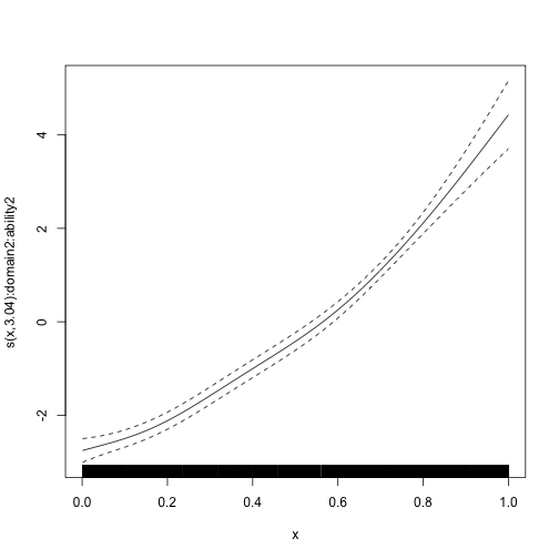
We can plot the estimated smooth terms, which recover their simulated ground truth very well.

plot_smooth(mod_byvar, scale = 0, select = 1)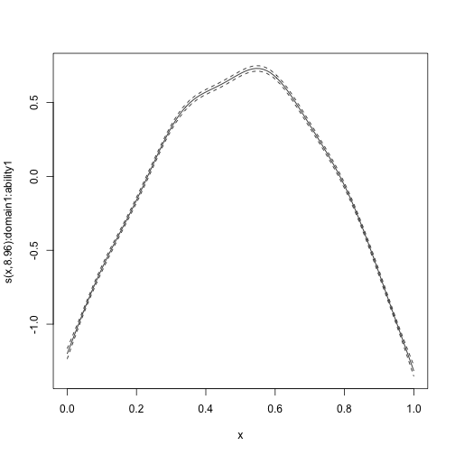

Estimated smooth term for domain 1 in model with domain 1 and domain 3.

plot_smooth(mod_byvar, scale = 0, select = 2)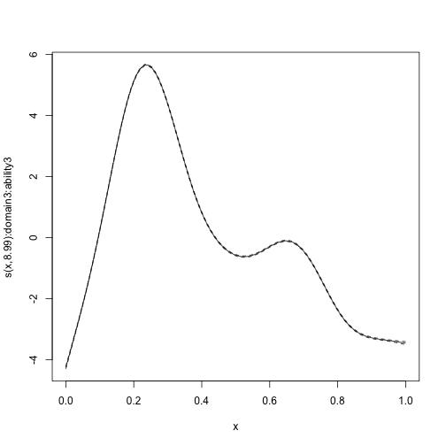

Estimated smooth term for domain 3 in model with domain 1 and domain 3.

Mixed Gaussian and Binomial Responses

Domain 1 has Gaussian responses and domain 2 has binomial responses, and we can model them jointly. For the sake of speed, we include only two items for each domain.

dat <- subset(cognition, domain %in% c(1, 2))

We also add indicator variables for the two domains.

dat <- cbind(
  dat,
  model.matrix(~ 0 + domain, data = dat)[, c("domain1", "domain2")]
  )

We define the loading matrix, now having two columns:

(lmat <- matrix(c(
    1, NA, NA, 0, 0,
    0, 0, 0, 1, NA
  ), ncol = 2))
#>      [,1] [,2]
#> [1,]    1    0
#> [2,]   NA    0
#> [3,]   NA    0
#> [4,]    0    1
#> [5,]    0   NA

Then we define the model. The smooth term is now sl(x, by = domain, factor = c("ability1", "ability2")), indicating that there should be a separate smooth term for each level of domain, and that the term should be multiplied by the loading “ability1” or “ability2”. Because this model has some convergence issues, we omit the timepoint-level random intercepts in this example.

mod_byvar_mixed <- galamm(
  formula = y ~ domain +
    sl(x, by = domain, factor = c("ability1", "ability2")) +
    (0 + domain1:ability1 + domain2:ability2 | id),
  data = dat,
  family = c(gaussian, binomial),
  family_mapping = ifelse(dat$domain == 1, 1L, 2L),
  load.var = "item",
  lambda = lmat,
  factor = c("ability1", "ability2"),
  control = galamm_control(
    optim_control = list(factr = 1e9, trace = 3, 
                         REPORT = 30, maxit = 1000)
  )
)
#> N = 12, M = 20 machine precision = 2.22045e-16
#> At X0, 0 variables are exactly at the bounds
#> At iterate     0  f=       8170.1  |proj g|=       2305.5
#> At iterate    30  f =       4726.2  |proj g|=        39.814
#> 
#> iterations 44
#> function evaluations 49
#> segments explored during Cauchy searches 44
#> BFGS updates skipped 0
#> active bounds at final generalized Cauchy point 0
#> norm of the final projected gradient 0.286444
#> final function value 4725.04
#> 
#> F = 4725.04
#> final  value 4725.035302 
#> converged

We can look at the model summary:

summary(mod_byvar_mixed)
#> GALAMM fit by maximum marginal likelihood.
#> Formula: y ~ domain + sl(x, by = domain, factor = c("ability1", "ability2")) +  
#>     (0 + domain1:ability1 + domain2:ability2 | id)
#>    Data: dat
#> Control: galamm_control(optim_control = list(factr = 1e+09, trace = 3,      REPORT = 30, maxit = 1000))
#> 
#>      AIC      BIC   logLik deviance df.resid 
#>   9476.1   9566.9  -4725.0  58315.3     7987 
#> 
#> Lambda:
#>         ability1      SE ability2      SE
#> lambda1   1.0000       .        .       .
#> lambda2   1.4082 0.01335        .       .
#> lambda3   0.2869 0.01040        .       .
#> lambda4        .       .   1.0000       .
#> lambda5        .       .   0.7996 0.05898
#> 
#> Random effects:
#>  Groups Name                  Variance Std.Dev. Corr
#>  id     domain1:ability1      2.4081   1.552        
#>         domain2:ability2      1.4827   1.218    0.40
#>  Xr.0   s(x):domain2:ability2 0.8501   0.922        
#>  Xr     s(x):domain1:ability1 2.2392   1.496        
#> Number of obs: 8000, groups:  id, 200; Xr.0, 8; Xr, 8
#> 
#> Fixed effects:
#>                          Estimate Std. Error z value  Pr(>|z|)
#> (Intercept)               0.04306    0.02253  1.9116 5.593e-02
#> domain2                   3.23013    0.16886 19.1290 1.449e-81
#> s(x):domain1:ability1Fx1 -0.08920    0.13855 -0.6438 5.197e-01
#> s(x):domain2:ability2Fx1  2.10045    0.47649  4.4082 1.042e-05
#> 
#> Approximate significance of smooth terms:
#>                         edf Ref.df   F p-value
#> s(x):domain1:ability1 7.865  7.865 880  <2e-16
#> s(x):domain2:ability2 3.036  3.036 285  <2e-16

We can plot the estimated smooth terms:

plot_smooth(mod_byvar_mixed, scale = 0, select = 1)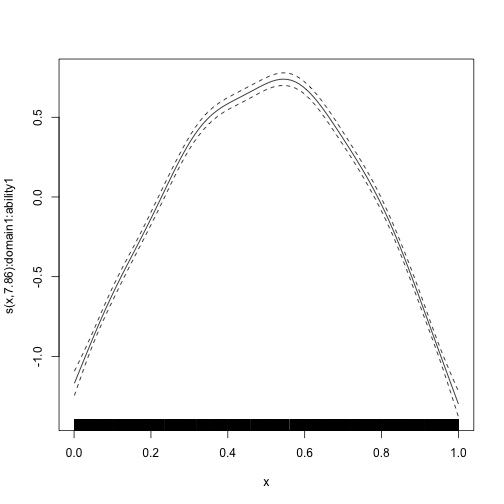

Estimated smooth term for domain 1 in mixed response model with domain 1 and domain 2.

plot_smooth(mod_byvar_mixed, scale = 0, select = 2)

Estimated smooth term for domain 1 in mixed response model with domain 1 and domain 2.

References

Hastie, Trevor, and Robert Tibshirani. 1993. “Varying-Coefficient Models.” Journal of the Royal Statistical Society: Series B (Methodological) 55 (4): 757–79. https://doi.org/10.1111/j.2517-6161.1993.tb01939.x.

Hodges, James S. 2013. Richly Parameterized Linear Models Additive, Time Series, and Spatial Models Using Random Effects. 1st ed. Chapman & Hall/CRC Texts in Statistical Science. Chapman & Hall.

Joe, Harry. 2008. “Accuracy of Laplace Approximation for Discrete Response Mixed Models.” Computational Statistics & Data Analysis 52 (12): 5066–74. https://doi.org/10.1016/j.csda.2008.05.002.

Sørensen, Øystein, Anders M. Fjell, and Kristine B. Walhovd. 2023. “Longitudinal Modeling of Age-Dependent Latent Traits with Generalized Additive Latent and Mixed Models.” Psychometrika 88 (2): 456–86. https://doi.org/10.1007/s11336-023-09910-z.

Wood, Simon N. 2017. Generalized Additive Models: An Introduction with R. 2nd ed. Chapman and Hall/CRC.