The cortical surface is not flat. Two regions can be close in Euclidean space—a straight line through the brain—yet far apart along the cortical sheet. This distinction matters whenever distance drives an analysis: computing spatial autocorrelation, selecting neighbours, or estimating how much cortex a region actually covers.
neuromapr provides tools for working with triangular surface meshes: building graphs, computing geodesic distances, calculating per-vertex surface areas, and converting between neuroimaging file formats.
Surface meshes
A cortical surface mesh consists of two pieces:
- Vertices: an n x 3 matrix of 3D coordinates, one row per point on the surface.
- Faces: an m x 3 matrix of integer indices, each row defining a triangle by referencing three vertices.
Together they describe the geometry. We build a small mesh by hand to make the examples concrete:
vertices <- matrix(c(
  0, 0, 0,
  1, 0, 0,
  0.5, 1, 0,
  1.5, 1, 0,
  0, 2, 0,
  1, 2, 0
), ncol = 3, byrow = TRUE)

faces <- matrix(c(
  1, 2, 3,
  2, 3, 4,
  3, 4, 6,
  3, 5, 6
), ncol = 3, byrow = TRUE)
Six vertices and four triangles forming a small irregular strip. Real cortical surfaces have tens of thousands of vertices, but the operations are the same.
Building a surface graph
make_surf_graph() converts a mesh into a weighted igraph
object. Each edge connects two vertices that share a triangle, and the
weight is the Euclidean distance between them.
g <- make_surf_graph(vertices, faces)
g
#> IGRAPH 4428296 U-W- 6 9 --
#> + attr: weight (e/n)
#> + edges from 4428296:
#> [1] 1--2 2--3 3--4 3--5 4--6 5--6 1--3 2--4 3--6
The graph captures the connectivity structure of the mesh—which vertices are adjacent and how far apart they are along the surface. It is the foundation for geodesic distance computation.
Here is what the graph looks like, using the vertex positions as layout coordinates. Edge labels show the Euclidean distance between connected vertices:
layout_xy <- vertices[, 1:2]
edge_weights <- round(
  igraph::E(g)$weight, 2
)

plot(
  g,
  layout = layout_xy,
  vertex.size = 20,
  vertex.color = "steelblue",
  vertex.label.color = "white",
  vertex.label.cex = 0.9,
  edge.label = edge_weights,
  edge.label.cex = 0.8,
  edge.color = "grey40",
  main = "Surface mesh graph"
)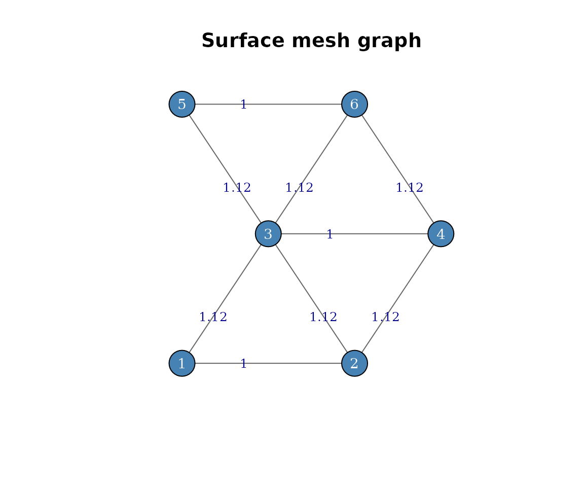
Surface graph of the toy mesh. Vertices are positioned at their x-y coordinates, edges are weighted by Euclidean distance.
On a real cortical surface, this graph has thousands of nodes and edges. The structure is the same: vertices connected by triangle edges, weights encoding surface distances.
Geodesic distances
Euclidean distance is a straight line through 3D space. Geodesic distance follows the surface, taking the shortest path along mesh edges. For a convoluted surface like the cortex, the two can differ substantially.
get_surface_distance() computes geodesic distances via
Dijkstra’s algorithm on the surface graph:
dmat <- get_surface_distance(vertices, faces)
dmat
#>          [,1]     [,2]     [,3]     [,4]     [,5]     [,6]
#> [1,] 0.000000 1.000000 1.118034 2.118034 2.236068 2.236068
#> [2,] 1.000000 0.000000 1.118034 1.118034 2.236068 2.236068
#> [3,] 1.118034 1.118034 0.000000 1.000000 1.118034 1.118034
#> [4,] 2.118034 1.118034 1.000000 0.000000 2.118034 1.118034
#> [5,] 2.236068 2.236068 1.118034 2.118034 0.000000 1.000000
#> [6,] 2.236068 2.236068 1.118034 1.118034 1.000000 0.000000
The result is a symmetric n x n matrix of shortest-path distances.
Partial distance matrices
Computing the full n x n matrix gets expensive for large meshes. If you only need distances from a subset of source vertices, pass them explicitly:
dmat_partial <- get_surface_distance(
  vertices, faces, source_vertices = c(1, 6)
)
dmat_partial
#>          [,1]     [,2]     [,3]     [,4]     [,5]     [,6]
#> [1,] 0.000000 1.000000 1.118034 2.118034 2.236068 2.236068
#> [2,] 2.236068 2.236068 1.118034 1.118034 1.000000 0.000000
A 2 x 6 matrix: distances from vertices 1 and 6 to all six vertices. For parcellation centroid computations and neighbourhood queries, this selective approach saves considerable time.
Euclidean vs geodesic
On a flat mesh the two distance measures coincide. On a folded cortex, geodesic distances are always greater than or equal to Euclidean, often substantially so for regions separated by a sulcus.
euclid <- as.matrix(dist(vertices))
geodesic <- get_surface_distance(vertices, faces)

max(abs(geodesic - euclid))
#> [1] 0.3152584
On our flat toy mesh the difference is zero. On real cortical surfaces, it is not.
Vertex areas
Each vertex on a surface mesh represents a patch of cortex. Knowing its area matters for area-weighted averaging and for understanding how much cortical surface a parcel covers.
vertex_areas() distributes each triangle’s area equally
among its three vertices:
areas <- vertex_areas(vertices, faces)
areas
#> [1] 0.1666667 0.3333333 0.6666667 0.3333333 0.1666667 0.3333333
sum(areas)
#> [1] 2
The total vertex area equals the total surface area of all triangles. Corner vertices (part of fewer triangles) get less area than interior vertices (shared by more triangles).
Checking the geometry
A sanity check: compute triangle areas directly and verify they sum to the same total.
tri_area <- function(v, f) {
  a <- v[f[1], ]
  b <- v[f[2], ]
  cc <- v[f[3], ]
  ab <- b - a
  ac <- cc - a
  cross <- c(
    ab[2] * ac[3] - ab[3] * ac[2],
    ab[3] * ac[1] - ab[1] * ac[3],
    ab[1] * ac[2] - ab[2] * ac[1]
  )
  0.5 * sqrt(sum(cross^2))
}

total_tri <- sum(vapply(
  seq_len(nrow(faces)),
  function(i) tri_area(vertices, faces[i, ]),
  numeric(1)
))

all.equal(sum(areas), total_tri)
#> [1] TRUE
Format conversions
Cortical surfaces come in many file formats. FreeSurfer uses its own
binary formats (.annot for parcellations,
.curv/.thickness/.sulc for
morphometry), while modern tools increasingly expect GIFTI. neuromapr
provides two conversion functions.
Annotation to GIFTI
annot_to_gifti() converts a FreeSurfer
.annot file (parcellation labels) to a GIFTI label
file:
annot_to_gifti("lh.aparc.annot", "lh.aparc.label.gii")Morphometry to GIFTI
fsmorph_to_gifti() converts FreeSurfer morphometry files
to GIFTI func files:
fsmorph_to_gifti("lh.thickness", "lh.thickness.func.gii")Both functions require the freesurferformats and
gifti packages. If no output path is given, they
replace the file extension automatically (.annot becomes
.label.gii, .curv becomes
.func.gii).
Resampling between coordinate spaces
Brain maps from different studies often live in different coordinate spaces (fsaverage vs fsLR) and at different mesh densities (32k vs 164k). Before you can compare them, they need to be in the same space at the same resolution.
transform_to_space() handles this resampling using
Connectome Workbench via the ciftiTools package:
transformed <- transform_to_space(
  "map.func.gii",
  target_space = "fsLR",
  target_density = "32k"
)
For pairwise comparisons, resample_images() aligns two
maps into a common space with a single call:
aligned <- resample_images(
  src = "map_a.func.gii",
  trg = "map_b.func.gii",
  src_space = "fsaverage",
  trg_space = "fsLR",
  strategy = "transform_to_trg"
)
Four strategies are available:
-
"downsample_only"— both maps already share a coordinate space; downsample the higher-density one. -
"transform_to_src"— bring the target into the source’s space. -
"transform_to_trg"— bring the source into the target’s space. -
"transform_to_alt"— bring both into a third space and density.
All resampling functions require Connectome Workbench
(wb_command). Use check_wb_command() to verify
it is installed and locatable:
Putting it together
A typical workflow that combines surface geometry with the rest of neuromapr:
- Load a surface mesh from a GIFTI
.surf.giifile. - Compute geodesic distances between parcel centroids.
- Feed that distance matrix into spatially-constrained null model generation.
centroids <- get_parcel_centroids(
  vertices, labels, method = "surface"
)
distmat <- as.matrix(dist(centroids))
nulls <- generate_nulls(
  parcel_data,
  method = "burt2020",
  distmat = distmat
)
For analyses where the distinction between Euclidean and geodesic distance matters—highly folded cortex, parcels separated by deep sulci—computing geodesic distances between centroids can produce more accurate null models.
References
Markello RD, Hansen JY, Liu Z-Q, et al. (2022). neuromaps: structural and functional interpretation of brain maps. Nature Methods, 19, 1472–1480. doi:10.1038/s41592-022-01625-w
Robinson EC, Jbabdi S, Glasser MF, et al. (2014). MSM: a new flexible framework for Multimodal Surface Matching. NeuroImage, 100, 414–426. doi:10.1016/j.neuroimage.2014.07.033