Getting Started with neuromapr

Two brain maps look correlated. But the brain is spatially autocorrelated—nearby regions tend to have similar values simply because they are neighbours. A standard correlation test ignores this structure, which inflates p-values and produces false positives.

neuromapr exists to answer one question honestly: is the similarity between two brain maps more than spatial structure alone would predict?

It generates surrogate maps that preserve the spatial autocorrelation of the original data, then measures where the real correlation falls in that null distribution. The framework follows Markello et al. (2022).

library(neuromapr)

Comparing two brain maps

The core workflow: load data, compare, interpret. We simulate two brain maps here to keep things self-contained, but in practice you would read real data from GIFTI or NIfTI files.

set.seed(42)
n <- 100
coords <- matrix(rnorm(n * 3), ncol = 3)
distmat <- as.matrix(dist(coords))

map_a <- rnorm(n)
map_b <- 0.4 * map_a + rnorm(n, sd = 0.8)

Two maps with a planted correlation around 0.4, plus a distance matrix describing the spatial layout. The simplest comparison:

result <- compare_maps(map_a, map_b, verbose = FALSE)
result
#> 
#> ── Brain Map Comparison
#> Method: pearson
#> r = 0.5302, p = 1.4e-08
#> n = 100

The r and parametric p tell the familiar story. But that p assumes independence between observations—an assumption the brain violates everywhere.

Adding a spatial null model

To get an honest p-value, we generate surrogate versions of map_a that preserve its spatial autocorrelation, then check whether the observed correlation is unusual against correlations with those surrogates.

neuromapr provides eight null model methods. For parcellated data with a distance matrix, variogram matching (burt2020) is a strong default:

result_null <- compare_maps(
  map_a, map_b,
  null_method = "burt2020",
  distmat = distmat,
  n_perm = 500L,
  seed = 1,
  verbose = FALSE
)
#> Generating burt2020 nulls ■■■■■■■■■■■■■■■■■                 53% | ETA:  4s
#> Generating burt2020 nulls ■■■■■■■■■■■■■■■■■■■■■■■■■■■       86% | ETA:  2s
result_null
#> 
#> ── Brain Map Comparison
#> Method: pearson
#> r = 0.5302, p = 1.4e-08
#> n = 100
#> ────────────────────────────────────────────────────────────────────────────────
#> Null model: burt2020 (500 permutations)
#> p_null = 0.002

The p_null value now accounts for spatial autocorrelation. If it remains small, the relationship between the two maps is unlikely to be an artifact of shared spatial structure.

Visualising the null distribution

The comparison object stores all null correlations, making it straightforward to see where the observed value falls:

null_df <- data.frame(r = result_null$null_r)
obs_r <- result_null$r

ggplot2::ggplot(null_df, ggplot2::aes(x = r)) +
  ggplot2::geom_histogram(
    bins = 30, fill = "steelblue", alpha = 0.7
  ) +
  ggplot2::geom_vline(
    xintercept = obs_r,
    linetype = "dashed", color = "red", linewidth = 1
  ) +
  ggplot2::labs(
    x = "Null correlation (r)",
    y = "Count"
  ) +
  ggplot2::theme_minimal()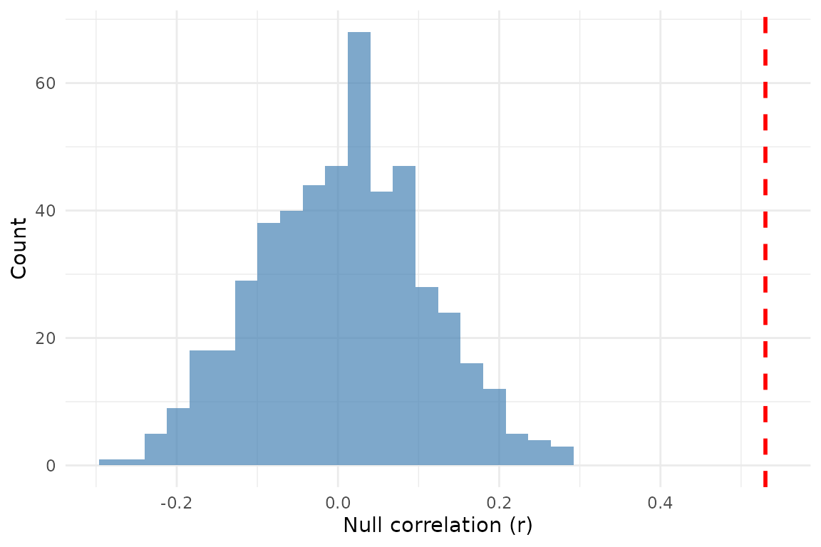

Null correlations from 500 variogram-matching surrogates. The dashed red line marks the observed correlation.

When the observed correlation sits well outside the null distribution, the relationship is more likely genuine. When it sits inside, spatial autocorrelation alone can explain the similarity.

Pre-computing null distributions

Generating nulls is the expensive part. If you want to compare the same map against several targets, generate once and reuse:

nulls <- generate_nulls(
  map_a,
  method = "moran",
  distmat = distmat,
  n_perm = 200L,
  seed = 42
)
nulls
#> 
#> ── Null Distribution
#> • Method: moran
#> • Permutations: 200
#> • Observations: 100

The null_distribution object has print, summary, plot, and as.matrix methods. The summary gives per-element null means and standard deviations. The plot method shows the null distribution for a chosen element:

plot(nulls, parcel = 1L)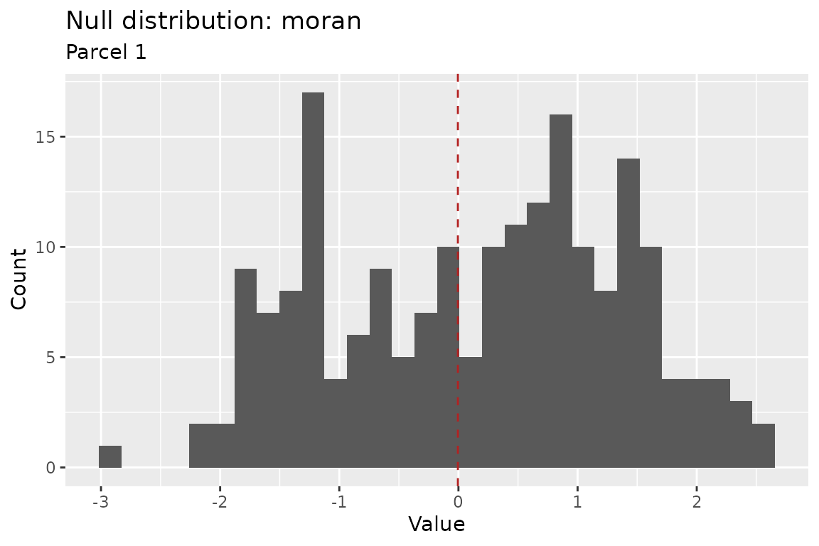

Built-in plot method for a null_distribution object.

Pass the pre-computed object to compare_maps():

compare_maps(map_a, map_b, nulls = nulls, verbose = FALSE)
#> 
#> ── Brain Map Comparison
#> Method: pearson
#> r = 0.5302, p = 1.4e-08
#> n = 100
#> ────────────────────────────────────────────────────────────────────────────────
#> Null model: moran (200 permutations)
#> p_null = 0.00498

No redundant computation when the same source map appears in multiple comparisons.

Working with real brain map files

In practice, brain maps live on disk. compare_maps() and read_brain_map_values() accept file paths directly:

values <- read_brain_map_values("cortical_thickness.func.gii")

result <- compare_maps(
  "path/to/map_a.func.gii",
  "path/to/map_b.func.gii",
  null_method = "moran",
  distmat = distmat
)

Both GIFTI (.func.gii) and NIfTI (.nii.gz) formats are supported. No separate reading step needed.

Accessing the neuromaps atlas collection

The neuromaps project curates a registry of published brain map annotations—PET receptor maps, gene expression, cortical thickness, and more. neuromapr provides direct access to this collection:

neuromaps_available()

neuromaps_available(source = "beliveau", tags = "pet")

Once you find the annotation you want, download it:

paths <- fetch_neuromaps_annotation(
  "abagen", "genepc1", "fsaverage",
  density = "10k"
)

Files are cached locally, so subsequent calls skip the download. The registry is fetched from the neuromaps GitHub repository and cached for the session.

Custom metrics with `permtest_metric()`

compare_maps() is built around correlation. For other metrics—mean absolute error, cosine similarity, anything that takes two vectors and returns a scalar—permtest_metric() provides the same null model machinery:

mae <- function(a, b) mean(abs(a - b))

result_mae <- permtest_metric(
  map_a, rnorm(n),
  metric_func = mae,
  n_perm = 200L,
  seed = 1
)
result_mae$observed
#> [1] 1.117007
result_mae$p_value
#> [1] 0.6517413

Add null_method for spatially-constrained surrogates instead of random permutation:

result_spatial <- permtest_metric(
  map_a, rnorm(n),
  metric_func = mae,
  n_perm = 200L,
  seed = 1,
  null_method = "burt2020",
  distmat = distmat
)
#> Generating burt2020 nulls ■■■■■■■■■■■■■■■■■■■■■■■■■         79% | ETA:  1s
result_spatial$p_value
#> [1] 0.8159204

Choosing a null model

The right model depends on your data:

Situation	Recommended method
Parcellated data with distance matrix	`"burt2020"` or `"moran"`
Vertex-level with sphere coordinates	`"spin_hungarian"` or `"alexander_bloch"`
Parcellated with sphere coordinates	`"baum"` or `"cornblath"`
Spatial autoregressive structure	`"burt2018"`

vignette("null-models") walks through each method in detail.

What comes next

This vignette covered the essential workflow: compare maps, generate spatially-constrained null distributions, and interpret results. From here:

vignette("null-models") dives into all eight null model methods and their assumptions.
vignette("parcellation") covers aggregating vertex data into parcels and parcel-level null models.
vignette("surface-geometry") explains geodesic distances, surface graphs, and vertex area calculations.

References

Markello RD, Hansen JY, Liu Z-Q, et al. (2022). neuromaps: structural and functional interpretation of brain maps. Nature Methods, 19, 1472–1480. doi:10.1038/s41592-022-01625-w