Choosing and Using Null Models

Correlating two brain maps is easy. Knowing whether that correlation means anything is the hard part.

The brain’s spatial autocorrelation means that even unrelated maps can appear correlated simply because nearby regions share similar values. Spatial null models address this by generating surrogate maps that preserve the spatial structure of the original while destroying the specific pattern of interest. If the observed correlation still stands out against these surrogates, you have evidence for a genuine relationship.

neuromapr implements eight null model methods. They differ in their assumptions, computational cost, and the kind of data they handle. This vignette walks through each one, explains when to reach for it, and names the tradeoffs plainly.

library(neuromapr)

The landscape

The eight methods split into three families.

Distance-based methods work with any distance matrix—Euclidean, geodesic, or custom. No coordinate system required, and they apply equally to parcellated and vertex-level data.

burt2020 — variogram matching
burt2018 — spatial autoregressive model
moran — Moran spectral randomization

Spin-based methods require spherical coordinates (one set per hemisphere) and operate on vertex-level data. They rotate the coordinates on the sphere, then reassign values based on proximity.

alexander_bloch — nearest-neighbour reassignment
spin_vasa — greedy sequential assignment
spin_hungarian — optimal (Hungarian) assignment

Parcel spin methods combine spin rotations with parcellation-level reassignment. They need both spherical coordinates and a parcellation scheme.

baum — maximum-overlap parcel assignment
cornblath — majority-vote parcel assignment

set.seed(42)
n <- 80
coords_3d <- matrix(rnorm(n * 3), ncol = 3)
distmat <- as.matrix(dist(coords_3d))

map_x <- rnorm(n)

Distance-based methods

Variogram matching (`burt2020`)

Burt et al. (2020) generate surrogates by randomly permuting the original values, then smoothing them at different spatial scales and selecting the surrogate whose variogram best matches the original. The result is a map with the same rank-order distribution and approximately the same distance-dependent spatial structure.

nulls_vario <- generate_nulls(
  map_x,
  method = "burt2020",
  distmat = distmat,
  n_perm = 100L,
  seed = 1
)
nulls_vario
#> 
#> ── Null Distribution
#> • Method: burt2020
#> • Permutations: 100
#> • Observations: 80

Variogram matching is the most general-purpose method. It makes no assumptions about the coordinate system, works on any distance matrix, and handles both parcellated and vertex-level data. The cost scales with the number of smoothing parameters tried per permutation, but for typical parcellation sizes (50–400 regions) it runs quickly.

When to use it: Default recommendation when you have a distance matrix and want minimal assumptions about the spatial generating process.

Spatial autoregressive model (`burt2018`)

Burt et al. (2018) take a generative approach: fit a spatial autoregressive (SAR) model to the data, then draw new samples from that model. The SAR model captures spatial autocorrelation through a weight matrix derived from distances and an estimated autocorrelation parameter.

nulls_sar <- generate_nulls(
  map_x,
  method = "burt2018",
  distmat = distmat,
  n_perm = 100L,
  seed = 1
)
nulls_sar
#> 
#> ── Null Distribution
#> • Method: burt2018
#> • Permutations: 100
#> • Observations: 80

The SAR model estimates two parameters: rho (spatial autocorrelation strength) and d0 (distance decay scale). These are stored in the result:

nulls_sar$params$rho
#>        wx 
#> -23.71389
nulls_sar$params$d0
#> [1] 3.463286

When to use it: When you believe the data follows an autoregressive spatial process and want surrogates drawn from that parametric model. More assumption-heavy than variogram matching, but computationally cheaper per surrogate once the parameters are estimated.

Moran spectral randomization (`moran`)

Wagner and Dray (2015) decompose the data onto Moran’s eigenvector maps—spatial eigenvectors of a weighted connectivity matrix—and then randomly perturb the coefficients. The "singleton" procedure flips the sign of each coefficient at random; the "pair" procedure applies random 2D rotations to pairs of coefficients with similar eigenvalues.

nulls_moran <- generate_nulls(
  map_x,
  method = "moran",
  distmat = distmat,
  n_perm = 100L,
  seed = 1,
  procedure = "singleton"
)
nulls_moran
#> 
#> ── Null Distribution
#> • Method: moran
#> • Permutations: 100
#> • Observations: 80

When to use it: When you want to preserve the spectral properties of the spatial autocorrelation rather than the variogram. The "pair" procedure is more conservative, preserving the eigenvalue spectrum more faithfully.

Spin-based methods

Spin tests work on a fundamentally different principle. Instead of generating synthetic data from a statistical model, they take the real data and rotate it on the cortical sphere. Values get reassigned to the original positions based on proximity to the rotated positions.

All spin methods require coordinates organized as a list with $lh and $rh components—one matrix per hemisphere. Each hemisphere rotates independently.

n_lh <- 40
n_rh <- 40
sphere_coords <- list(
  lh = matrix(rnorm(n_lh * 3), ncol = 3),
  rh = matrix(rnorm(n_rh * 3), ncol = 3)
)

vertex_data <- rnorm(n_lh + n_rh)

Original spin test (`alexander_bloch`)

The method that started it all (Alexander-Bloch et al., 2018). After rotating coordinates, each rotated vertex maps to the nearest original vertex. Multiple rotated vertices can map to the same original, so some values get duplicated while others are dropped.

nulls_ab <- null_alexander_bloch(
  vertex_data, sphere_coords,
  n_perm = 100L, seed = 1
)
nulls_ab
#> 
#> ── Null Distribution
#> • Method: alexander_bloch
#> • Permutations: 100
#> • Observations: 80

The simplest spin test and the fastest. The tradeoff: the many-to-one mapping distorts the value distribution. If preserving the distribution matters, the Hungarian variant is more appropriate.

Greedy assignment (`spin_vasa`)

Vasa et al. (2018) proposed one-to-one greedy assignment: iterate through vertices in order, assigning each to the nearest available (unassigned) rotated vertex. Every value appears exactly once, but assignment quality depends on vertex ordering.

nulls_vasa <- null_spin_vasa(
  vertex_data, sphere_coords,
  n_perm = 100L, seed = 1
)
nulls_vasa
#> 
#> ── Null Distribution
#> • Method: spin_vasa
#> • Permutations: 100
#> • Observations: 80

Optimal assignment (`spin_hungarian`)

Markello and Misic (2021) showed that optimal (Hungarian) assignment removes the ordering bias of the greedy approach. It minimizes total reassignment distance globally, producing the best possible one-to-one mapping between original and rotated positions.

nulls_hung <- null_spin_hungarian(
  vertex_data, sphere_coords,
  n_perm = 100L, seed = 1
)
nulls_hung
#> 
#> ── Null Distribution
#> • Method: spin_hungarian
#> • Permutations: 100
#> • Observations: 80

The Hungarian algorithm requires the clue package and runs in cubic time in the number of vertices. Slower than the greedy approach, but strictly better assignments.

When to use it: The recommended spin method for vertex-level data when you want one-to-one assignment and can afford the extra computation.

Parcel spin methods

When your data is parcellated—one value per brain region rather than per vertex—the spin rotation still happens at vertex level, but the reassignment happens at the parcel level. This requires both sphere coordinates (for the rotation) and a parcellation vector (to know which vertices belong to which parcel).

n_parcel_lh <- 340
n_parcel_rh <- 340
parcel_coords <- list(
  lh = matrix(rnorm(n_parcel_lh * 3), ncol = 3),
  rh = matrix(rnorm(n_parcel_rh * 3), ncol = 3)
)
parcellation <- rep(1:68, each = 10)
parcel_data <- rnorm(68)

Maximum overlap (`baum`)

Baum et al. (2020) proposed that after rotating and reassigning vertices to their nearest neighbours, each original parcel takes the value of whichever rotated parcel has the most vertex overlap with it. If most vertices in parcel 3 now carry the label of parcel 7 after rotation, parcel 3 gets parcel 7’s value.

nulls_baum <- null_baum(
  parcel_data, parcel_coords, parcellation,
  n_perm = 50L, seed = 1
)
nulls_baum
#> 
#> ── Null Distribution
#> • Method: baum
#> • Permutations: 50
#> • Observations: 68

Majority vote (`cornblath`)

Cornblath et al. (2020) introduced a refinement: each rotated vertex first receives the label of its nearest non-medial-wall original vertex. Parcels are then reassigned by majority vote among the resulting vertex labels. This handles the medial wall more gracefully than Baum’s method, since rotated vertices that land on the medial wall get interpolated to the nearest valid region instead of being lost.

nulls_corn <- null_cornblath(
  parcel_data, parcel_coords, parcellation,
  n_perm = 50L, seed = 1
)
nulls_corn
#> 
#> ── Null Distribution
#> • Method: cornblath
#> • Permutations: 50
#> • Observations: 68

When to use it: Prefer Cornblath over Baum when your parcellation includes medial wall vertices (labeled 0 or NA), which is the common case for standard atlases.

Comparing null distributions visually

A practical way to understand what each method does: look at the surrogate values it produces. Here we compare the first 50 surrogates from two methods on the same data:

df <- data.frame(
  value = c(
    as.vector(nulls_vario$nulls[, 1:50]),
    as.vector(nulls_moran$nulls[, 1:50])
  ),
  method = rep(
    c("burt2020 (variogram)", "moran (spectral)"),
    each = n * 50
  )
)

ggplot2::ggplot(df, ggplot2::aes(x = value)) +
  ggplot2::geom_density(fill = "steelblue", alpha = 0.5) +
  ggplot2::facet_wrap(~method) +
  ggplot2::geom_density(
    data = data.frame(value = map_x),
    color = "red", linetype = "dashed", linewidth = 0.8
  ) +
  ggplot2::labs(x = "Value", y = "Density") +
  ggplot2::theme_minimal()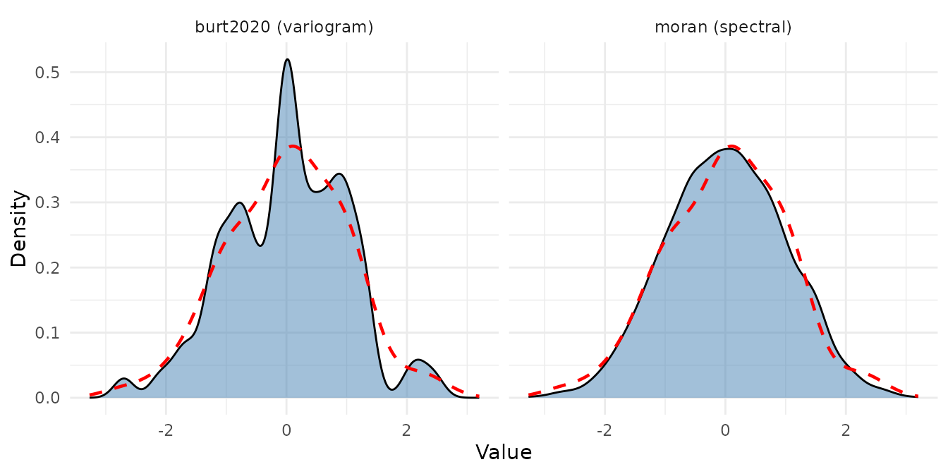

Surrogate distributions from variogram-matching (left) and Moran spectral randomization (right). The dashed red line is the original data distribution.

The red dashed line shows the original data distribution. Good surrogates should have a similar overall distribution (same value pool) but different spatial arrangements.

Using `permtest_metric()` for custom metrics

compare_maps() is built around correlation. If you need a different metric—mean absolute error, cosine similarity, whatever—use permtest_metric() with any function that takes two vectors and returns a scalar:

mae <- function(a, b) mean(abs(a - b))

result <- permtest_metric(
  map_x, rnorm(n),
  metric_func = mae,
  n_perm = 200L,
  seed = 1
)
result$observed
#> [1] 1.271935
result$p_value
#> [1] 0.06467662

Pass null_method for spatially-constrained surrogates instead of random permutation:

result_spatial <- permtest_metric(
  map_x, rnorm(n),
  metric_func = mae,
  n_perm = 200L,
  seed = 1,
  null_method = "burt2020",
  distmat = distmat
)
#> Generating burt2020 nulls ■■■■■■■■■■■■■■■■■■■■■■■■■■■■■     94% | ETA:  0s
result_spatial$p_value
#> [1] 0.9701493

Building custom null distributions

If you generate surrogates through some other means—your own algorithm, or an external tool—you can wrap them in a null_distribution object to use with the rest of neuromapr:

custom_nulls <- matrix(rnorm(n * 50), nrow = n, ncol = 50)
nd <- new_null_distribution(
  custom_nulls,
  method = "custom",
  observed = map_x
)
nd
#> 
#> ── Null Distribution
#> • Method: custom
#> • Permutations: 50
#> • Observations: 80
summary(nd)
#> $method
#> [1] "custom"
#> 
#> $n_perm
#> [1] 50
#> 
#> $n
#> [1] 80
#> 
#> $null_mean
#>  [1]  0.172104151 -0.191992723  0.251970813 -0.089094615  0.005477459
#>  [6] -0.116195137  0.029984331 -0.140259990 -0.064275614  0.088438311
#> [11]  0.056367310 -0.020295656  0.107279055  0.061478744  0.028883291
#> [16] -0.124575306  0.116467203 -0.123478121  0.171316602 -0.320174552
#> [21] -0.101879306 -0.034256823  0.008095363 -0.166195389 -0.040686955
#> [26] -0.295944980 -0.158414959 -0.111692689  0.392321021 -0.118694798
#> [31]  0.271417483 -0.191272504 -0.075820891 -0.111577630 -0.050967630
#> [36] -0.079687220 -0.140829048  0.158767493  0.081045021 -0.155888319
#> [41]  0.007091098 -0.062884388 -0.015538874 -0.033575553  0.023571868
#> [46]  0.013706066 -0.098295867  0.070025536 -0.093369574 -0.158416906
#> [51] -0.101856761  0.174691830 -0.076514622  0.123438021 -0.088212642
#> [56] -0.027671164 -0.078829748 -0.000737019  0.192288238 -0.028717724
#> [61] -0.193521709 -0.096663995 -0.364682514 -0.118517540  0.173511672
#> [66]  0.038468503 -0.018096533  0.037188074 -0.072948543  0.110674743
#> [71] -0.012996721  0.385415691 -0.300242799 -0.180628593 -0.117331838
#> [76] -0.034619084 -0.046325206  0.115086854  0.063031223  0.011060466
#> 
#> $null_sd
#>  [1] 0.7654993 0.9942784 0.9519727 1.0154925 0.9496659 1.0151536 1.0555189
#>  [8] 1.0660867 0.7623388 1.0055644 1.0180568 1.1340219 1.0456170 0.9969020
#> [15] 1.0009006 0.9792541 0.8110526 0.9909006 1.0164368 0.9235815 0.7962349
#> [22] 1.1881215 1.0004296 0.9874878 1.0326598 1.0308064 1.0819856 0.9828809
#> [29] 1.0112092 1.0589840 0.8547717 0.9703791 0.9335735 1.0952835 0.9120905
#> [36] 0.9003178 1.0359273 0.8367114 0.9864675 0.8479680 0.9043361 0.8392895
#> [43] 0.9475172 0.9605337 1.0278489 1.1326076 1.0304862 0.9623529 1.0188185
#> [50] 0.9403089 0.9975970 1.0924189 0.9934468 1.0437525 0.8306250 0.9374071
#> [57] 0.8854729 0.9913599 0.9753211 1.1380680 1.0087496 1.0851607 0.9781671
#> [64] 0.9254884 0.9508746 1.0426264 1.1076917 0.9434507 1.0203667 1.0087854
#> [71] 1.0423534 1.1013250 0.8159138 1.0535077 0.8889507 1.0989718 0.9004764
#> [78] 1.0396253 0.9796304 0.8743524
#> 
#> $observed
#>  [1] -0.729217277  0.998068909  1.258481665  1.248863689 -1.380637050
#>  [6]  2.049960694  1.016872830 -0.026717464  0.703607779 -0.971385229
#> [11] -1.096156242  0.049050451 -1.198495857  0.190018999  1.297705900
#> [16] -1.033873723 -0.738440754  0.046563939 -1.017596120 -0.383283960
#> [21]  0.872755412  0.969545014  0.383846665 -1.851555663 -0.053996737
#> [26]  1.064773214  0.813195037 -0.190816474 -2.699929809  0.060966639
#> [31]  0.573751697  0.045803580  0.157412540  0.431565373 -0.396549736
#> [36]  1.309978226  0.470393400 -1.242670271  1.381575456  1.204458937
#> [41]  0.824073964 -1.662629402 -0.569306344  0.635513817  0.043722008
#> [46]  0.348012304  2.459593549 -0.818380324 -2.113200115  0.273695272
#> [51] -0.687596841  0.446041053 -0.812384724  2.212055480 -0.123705972
#> [56] -0.477335506 -0.166261491  0.862563384  0.097340485 -1.625616739
#> [61] -0.004620768  0.760242168  0.038990913  0.735072142 -0.146472627
#> [66] -0.057887335  0.482369466  0.992943637 -1.246395498 -0.033487525
#> [71] -0.070962181 -0.758920654 -1.034359361 -0.630731954  0.586807720
#> [76] -0.416322656 -0.784887810  0.163416319 -1.236714235  1.045873776

The new_null_distribution() constructor produces an object that works with compare_maps(nulls = ...), plot(), summary(), and as.matrix().

Decision guide

When faced with a choice, these questions narrow it down:

Do you have spherical coordinates? If not, use a distance-based method (burt2020, burt2018, or moran).
Is your data parcellated or vertex-level? Parcellated + sphere coords points to baum or cornblath. Vertex-level + sphere coords points to spin_hungarian or alexander_bloch.
Does the medial wall matter? If your parcellation has medial wall vertices, cornblath handles them more carefully than baum.
Do you want a parametric model? burt2018 fits an explicit SAR model. moran preserves spectral properties. burt2020 is distribution-free.
Computational budget? alexander_bloch and burt2018 are the fastest. spin_hungarian and burt2020 are the slowest (but often the most principled for their respective data types).

References

Alexander-Bloch AF, Shou H, Liu S, et al. (2018). On testing for spatial correspondence between maps of human brain structure and function. NeuroImage, 175, 111–120.

Baum GL, Cui Z, Roalf DR, et al. (2020). Development of structure–function coupling in human brain networks during youth. PNAS, 117, 21854–21861.

Burt JB, Demirtas M, Eckner WJ, et al. (2018). Hierarchy of transcriptomic specialization across human cortex captured by structural connectivity. Nature Neuroscience, 21, 1251–1259.

Burt JB, Helmer M, Shinn M, et al. (2020). Generative modeling of brain maps with spatial autocorrelation. NeuroImage, 220, 117038.

Cornblath EJ, Ashourvan A, Kim JZ, et al. (2020). Temporal sequences of brain activity at rest are constrained by white matter structure and modulated by cognitive demands. Communications Biology, 3, 590.

Markello RD, Misic B (2021). Comparing spatial null models for brain maps. NeuroImage, 236, 118052.

Vasa F, Seidlitz J, Romero-Garcia R, et al. (2018). Adolescent tuning of association cortex in human structural brain networks. Cerebral Cortex, 28, 3293–3303.

Wagner HH, Dray S (2015). Generating spatially constrained null models for irregularly spaced data using Moran spectral randomization methods. Methods in Ecology and Evolution, 6, 1169–1178.

The landscape

Distance-based methods

Variogram matching (burt2020)

Spatial autoregressive model (burt2018)

Moran spectral randomization (moran)