Introduction
Introduction.RmdThe galamm packages estimates generalized additive
latent and mixed models (GALAMMs). GALAMMs are described in Sørensen, Fjell, and Walhovd (2023) as an
extension of generalized linear latent and mixed models (GLLAMMs) (Rabe-Hesketh, Skrondal, and Pickles 2004).
In this vignette we demonstrate basic model formulation.
head(dat1)
#>   id  item         y         x
#> 1  1 item1  4.516161 0.5324675
#> 2  1 item2  8.955929 0.5324675
#> 3  1 item3  1.774563 0.5324675
#> 4  2 item1 10.144956 0.6560528
#> 5  2 item2 19.633269 0.6560528
#> 6  2 item3  4.525468 0.6560528
The dataset illustrates measurements of a latent response variable. The variables are
-
id: an identifier for the study subjects. -
item: an identifier for one of three items which measure an underlying latent trait of interest. -
y: the measurement of the given item. -
x: a predictor variable.
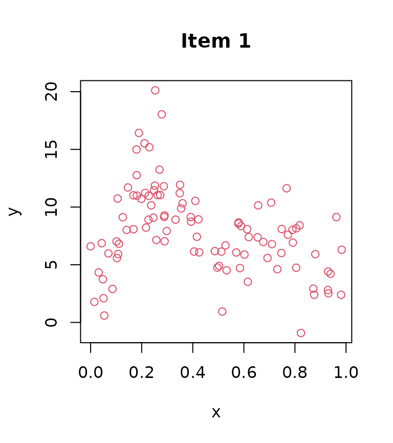
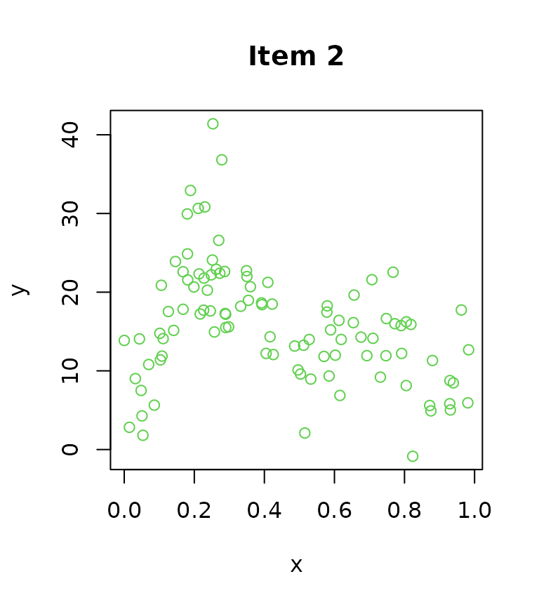
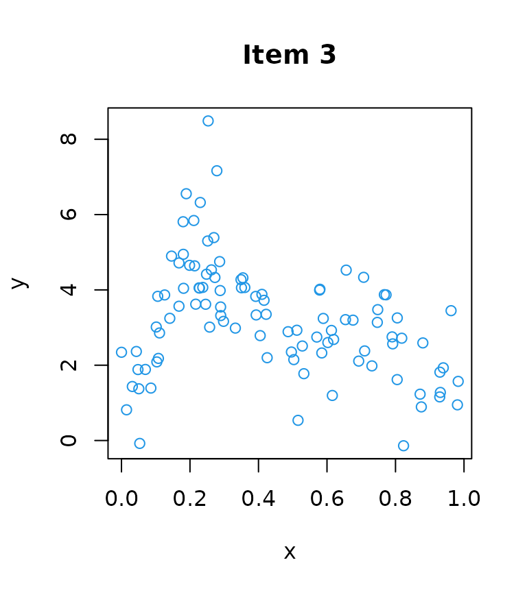
The plot below shows the measurements of each item.
sdat <- split(dat1, f = dat1$item)
for(i in seq_along(sdat)){
  plot(sdat[[i]]$x, sdat[[i]]$y, col = i + 1,
       xlab = "x", ylab = "y",
       main = paste("Item", i))
}


Model definition
Letting \(y_{ij}\) denotes the \(i\)th measurement of the \(j\)th subject, we assume the measurement part
\[y_{ij} = \beta_{0} + \eta_{j} \boldsymbol{\lambda}^{T} \boldsymbol{\delta}_{ij} + \epsilon_{ij}\]
where \(\boldsymbol{\delta}_{ij}\) is a vector whose \(k\)th element equals 1 if the \(i\)th measurement of the \(j\)th subject is a measurement of item \(k\), and \(\boldsymbol{\lambda} = (1, \lambda_{2}, \lambda_{3})^{T}\) is a vector of factor loadings, whose first element is set to 1 for identifiability. Furthermore, \(\eta_{j}\) denotes a latent variable for subject \(j\), assumed identical across all three items, and \(\epsilon_{ij} \sim N(0, \sigma^{2})\) is the residual term.
Next, the structural part relates the latent variables to the predictor variables,
\[\eta_{j} = f(x_{j}) + \zeta_{j}\]
where \(x_{j}\) is a predictor variable for subject \(j\) which does not vary within subjects, and \(\zeta_{j} \sim N(0, \psi)\) is a disturbance term (random intercept).
Plugging the structural model into the measurement model yields the reduced form
\[y_{ij} = \beta_{0} + f(x_{j}) \boldsymbol{\lambda}^{T} \boldsymbol{\delta}_{ij} + \zeta_{j} \boldsymbol{\lambda}^{T} \boldsymbol{\delta}_{ij} + \epsilon_{ij}\]
At fixed values of \(\boldsymbol{\lambda}\), the reduced form
defines a generalized additive mixed model (GAMM) (Wood 2017) with varying coefficient term \(f(x_{j}) \boldsymbol{\lambda}^{T}
\boldsymbol{\delta}_{ij}\) and random effect term \(\zeta_{j} \boldsymbol{\lambda}^{T}
\boldsymbol{\delta}_{ij}\). Identifying this lets us use profile
likelihood estimation similar to what Jeon and
Rabe-Hesketh (2012) proposed for a subset of GLLAMMs, and Rockwood and Jeon (2019) implemented in the R
package PLmixed. The galamm package instead
maximizes the Laplace approximate marginal likelihood directly, as
described in another vignette.